Part A: Image Warping and Mosaicing

In Part A of this project, I explore image warping and mosaicing through four main components: shooting photographs with projective transformations, recovering homographies from point correspondences, warping images using nearest neighbor and bilinear interpolation, and blending images into seamless mosaics. This foundational work prepares for the automated feature detection and matching in Part B.

Part A.1: Shoot and Digitize Pictures

For this part, I captured multiple sets of photographs with projective transformations between them. The key requirement is to fix the center of projection (COP) and rotate the camera while capturing photos. This creates the perspective transformations needed for mosaicing.

I focused on scenes with significant overlap (40-70%) and rich detail to make registration easier. The photographs were taken as close together in time as possible to minimize lighting changes and subject movement. I used my iPhone to take the photographs, without a tripod (unfortunately I don't have one). The center of projection for many of the images I took were approximately fixed, and the camera was rotated to capture the scene. My hands are not very steady, so the images are not perfectly still, but they are close.

Two images of the Anchor House taken from next to Li Ka Shing, with approximately fixed center of projection and significant overlap.

Two images of the Memorial Glade in Berkeley taken from the Grimes Engineering Center, with approximately fixed center of projection and significant overlap.

Two images with the Hearst Mining Circle peeking through, taken from next to Cory, with fixed center of projection and significant overlap.

Thirteen images of the glade from Grimes Engineering Center, with approximately fixed center of projection and significant overlap between each successive image.

Part A.2: Recover Homographies

Before warping images into alignment, I need to recover the parameters of the transformation between each pair of images. The transformation is a homography: $\mathbf{p'} = H\mathbf{p}$, where $H$ is a 3×3 matrix with 8 degrees of freedom (the lower right corner is set to 1 for scaling). The minimum number of point correspondences needed to recover the homography is 4, but we want as many as possible to get a more accurate homography, since if there are too few, a single pixel error in one of the points will throw off the entire homography. Correspondence points were chosen by hand using a selection tool written by a prior student and provided to us in the project instructions.

I implemented the function computeH(im1_pts, im2_pts) where the input parameters are n×2 matrices holding the (x,y) locations of n point correspondences from two images, and H is the recovered 3×3 homography matrix. Below is the mathematical derivation for the least squares problem we are solving to recover the homography matrix, as well as the pseudocode for the code implementation. We use numpy.linalg.lstsq to solve the least squares problem.

Mathematical Derivation

For a homography transformation, we have:

Expanding the matrix multiplication gives us homogeneous coordinates:

Converting back to Cartesian coordinates by dividing by $w$:

Cross-multiplying to eliminate the denominators:

Rearranging into linear form:

For each point correspondence $(x_i, y_i) \leftrightarrow (x'_i, y'_i)$, we get two linear equations. We can write this as a matrix equation $\mathbf{A}\mathbf{h} = \mathbf{b}$:

For an overdetermined system (n > 4 correspondences), we solve using least squares:

def computeH(im1_pts, im2_pts):
    1. Initialize matrix A (2n × 8) and vector b (2n × 1) following the equations above.
    
    2. For each point correspondence (x_i, y_i) ↔ (x'_i, y'_i):
       - Fill row 2i of A with: [x, y, 1, 0, 0, 0, -x*x', -y*x']
       - Fill row 2i+1 of A with: [0, 0, 0, x, y, 1, -x*y', -y*y']
       - Set b[2i] = x' and b[2i+1] = y'
    
    3. Solve the least squares problem Ah = b:
       h = np.linalg.lstsq(A, b)[0]
    
    4. Reshape h into 3×3 homography matrix:
       H = [[h[0], h[1], h[2]],
            [h[3], h[4], h[5]], 
            [h[6], h[7], 1.0]]
    
    5. Return H

Recovered Homography Matrices

After solving the least squares system $\mathbf{A}\mathbf{h} = \mathbf{b}$ using np.linalg.lstsq, we reshape the solution vector $\mathbf{h}$ into the 3×3 homography matrix. Here are the recovered homographies for each image pair:

Point correspondences for the left vs right anchor house images, 51 points were selected.

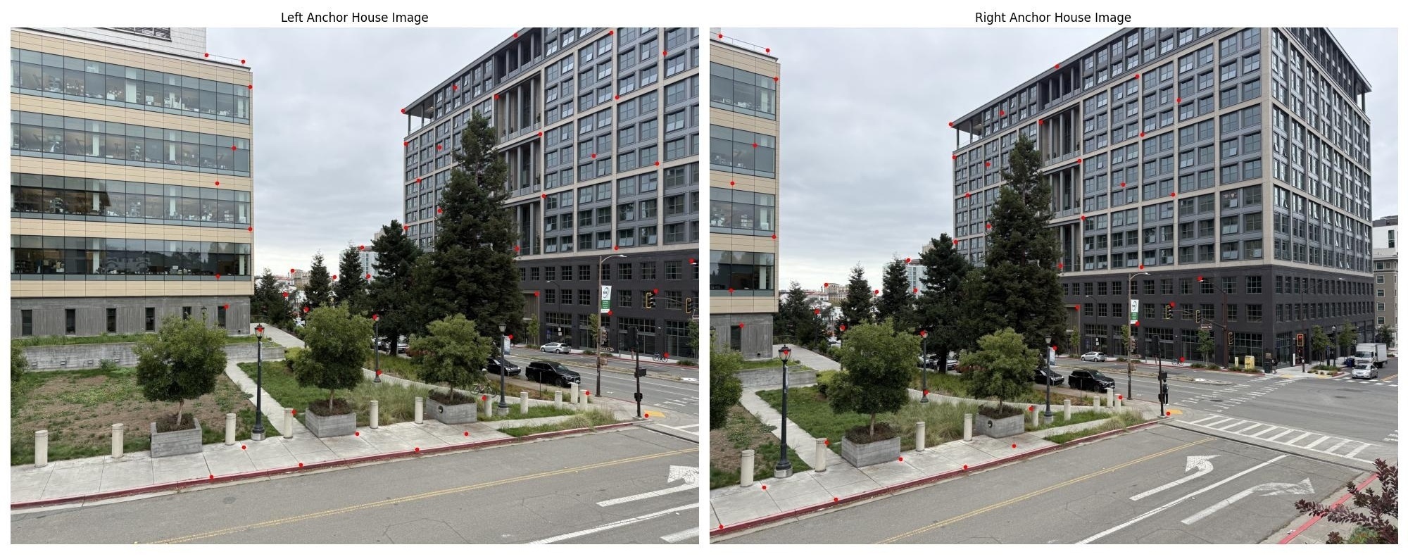
Left vs Right Anchor House - Homography Matrix:

Point correspondences for the left vs right glade images, 41 points were selected.

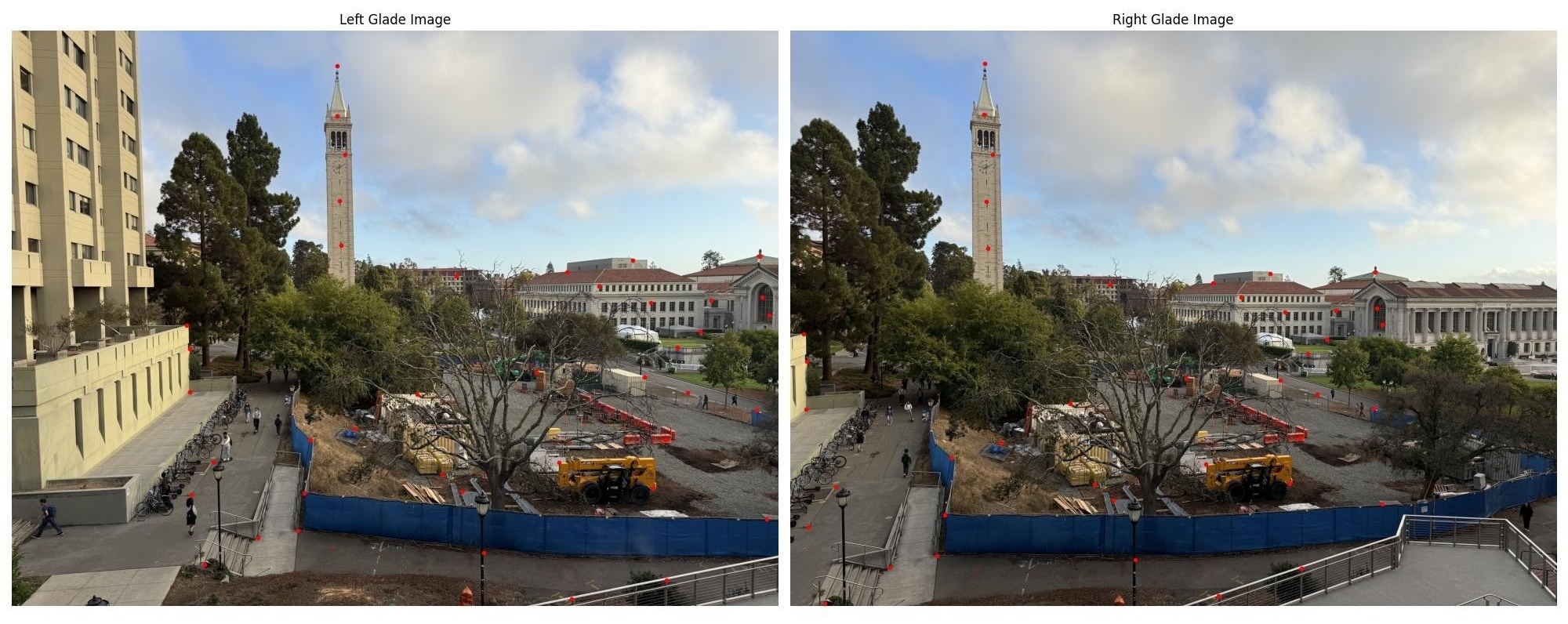
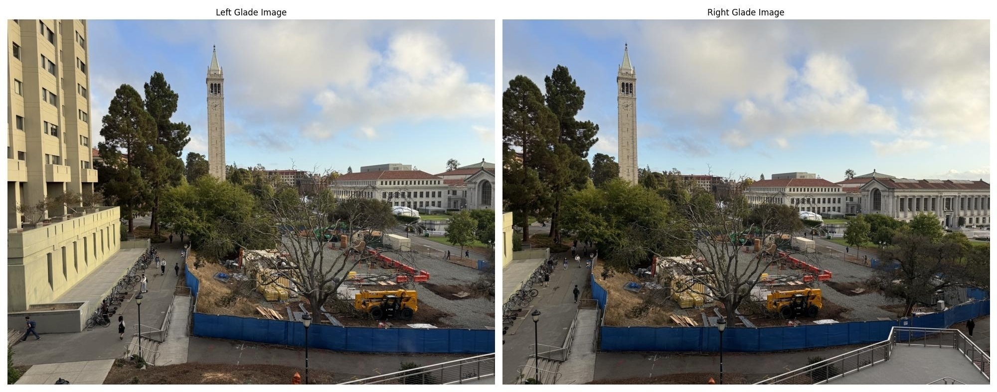
Left vs Right Glade - Homography Matrix:

Point correspondences for the left vs right mining circle images, 47 points were selected.

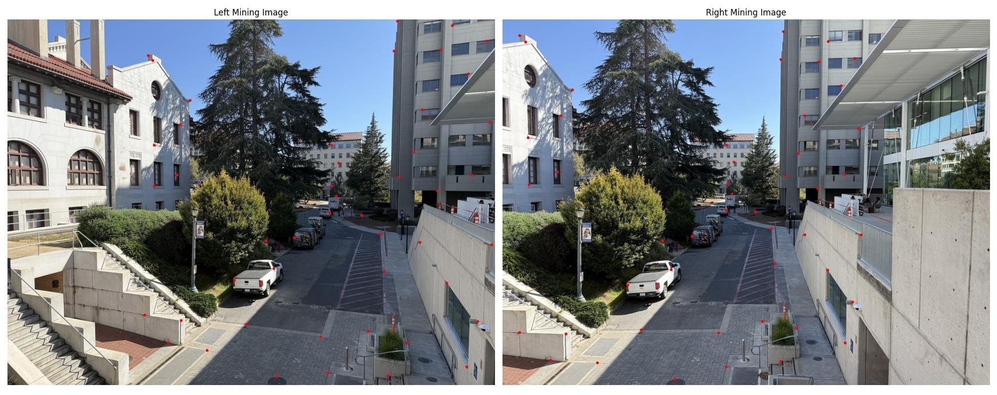
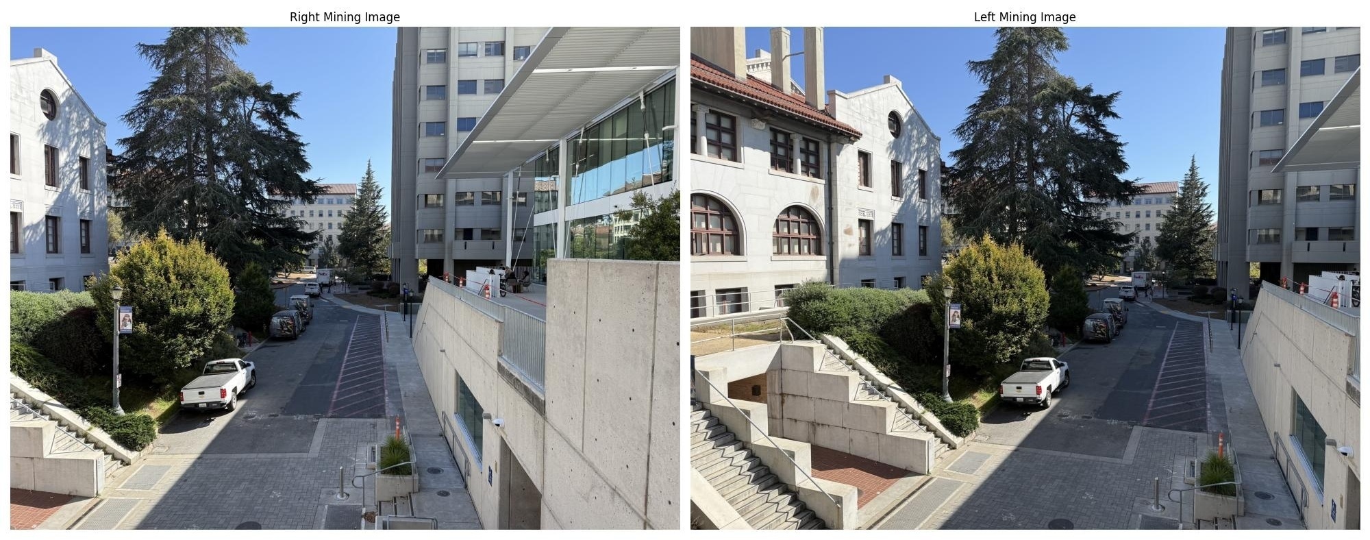
Left vs Right Mining - Homography Matrix:

Part A.3: Warp the Images

Using the computed homographies, I can now warp images towards a reference image. I implemented two interpolation methods from scratch using inverse warping to avoid holes in the output:

• Nearest Neighbor Interpolation: Round coordinates to the nearest pixel value
• Bilinear Interpolation: Use weighted average of four neighboring pixels

Implementation Details

1. Output Canvas Size Calculation

Both warping functions begin by determining the size of the output canvas needed to contain the entire warped image:

# Transform the four corners of the input image
corner_points = np.array([[0, 0, 1], [w, 0, 1], [w, h, 1], [0, h, 1]])
warped_corners = H @ corner_points.T
warped_corners = warped_corners[:2, :] / warped_corners[2, :]  # Convert to Cartesian

# Find bounding box of warped corners
min_x, max_x = np.floor(warped_corners[0].min()), np.ceil(warped_corners[0].max())
min_y, max_y = np.floor(warped_corners[1].min()), np.ceil(warped_corners[1].max())
out_h, out_w = max_y - min_y, max_x - min_x

This ensures the output image is large enough to contain the entire warped result, accounting for rotations and perspective distortions that might expand the image boundaries.

2. Inverse Warping Strategy

Both implementations use inverse warping to avoid holes in the output image. For each pixel in the output image, we:

1. Convert output coordinates to global coordinates: (x_glob, y_glob) = (out_x + min_x, out_y + min_y)
2. Apply inverse homography: H⁻¹ × [x_glob, y_glob, 1]ᵀ
3. Convert back to Cartesian coordinates by dividing by the homogeneous coordinate
4. Sample the input image at the resulting location using interpolation

3. Nearest Neighbor Interpolation

# Convert homogeneous coordinates back to Cartesian and round
x_src = int(round(original_pt[0] / original_pt[2]))
y_src = int(round(original_pt[1] / original_pt[2]))

# Simple bounds check and direct pixel copy
if 0 <= x_src < w and 0 <= y_src < h:
    warped_image[out_y, out_x] = im[y_src, x_src]

Nearest neighbor is the simplest interpolation method. It rounds the source coordinates to the nearest integer pixel location and directly copies that pixel's value. This is fast but can produce blocky artifacts, especially when significantly stretching and warping images.

4. Bilinear Interpolation

# Keep fractional coordinates for interpolation
x_src = original_pt[0] / original_pt[2]
y_src = original_pt[1] / original_pt[2]

# Find the four surrounding pixels
x_lower, y_lower = int(np.floor(x_src)), int(np.floor(y_src))
x_upper, y_upper = x_lower + 1, y_lower + 1

# Calculate interpolation weights
x_change = x_src - x_lower  # fractional part in x
y_change = y_src - y_lower  # fractional part in y

# Weighted average of four neighboring pixels
warped_image[out_y, out_x] = (1 - x_change) * (1 - y_change) * im[y_lower, x_lower] + \
                             x_change * (1 - y_change) * im[y_lower, x_upper] + \
                             (1 - x_change) * y_change * im[y_upper, x_lower] + \
                             x_change * y_change * im[y_upper, x_upper]

Bilinear interpolation provides much smoother results by computing a weighted average of the four nearest pixels. The weights are determined by the fractional parts of the source coordinates:

• Top-left weight: $(1 - x_{frac}) \times (1 - y_{frac})$
• Top-right weight: $x_{frac} \times (1 - y_{frac})$
• Bottom-left weight: $(1 - x_{frac}) \times y_{frac}$
• Bottom-right weight: $x_{frac} \times y_{frac}$

This produces smoother images with less aliasing, especially important for rotations and scaling operations.

5. Boundary Handling

Both implementations include careful boundary checking to ensure we only sample pixels that exist in the source image. Pixels that map outside the source image boundaries are left as zeros (black), creating a natural alpha mask effect.

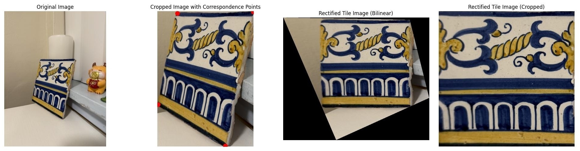
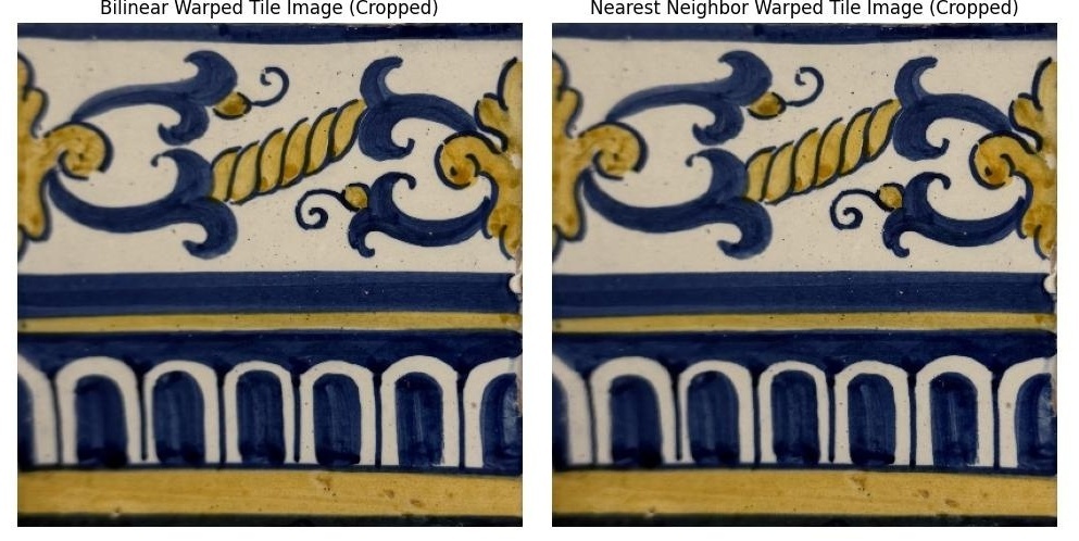
Rectification Results

To test the homography and warping implementation, I performed rectification on images containing rectangular objects. By defining correspondences between a tilted rectangle and a perfect square, I can verify that the warping correctly transforms perspective distortions. First, we get the correspondence points for the tilted rectangle from our correspondence tool. We crop the image to a small padded distance around the maximum width and height of the selected points. The second set of points can just be set to the four corners of a random rectangle of your choosing. Then, we calculate the homography matrix using these two sets of points and warp the image using our different interpolation methods.

Rectification of a poster depicting Keith Haring's "Men Holding a Heart" using bilinear interpolation.

Comparison of rectification results using bilinear and nearest neighbor interpolation of the same image.

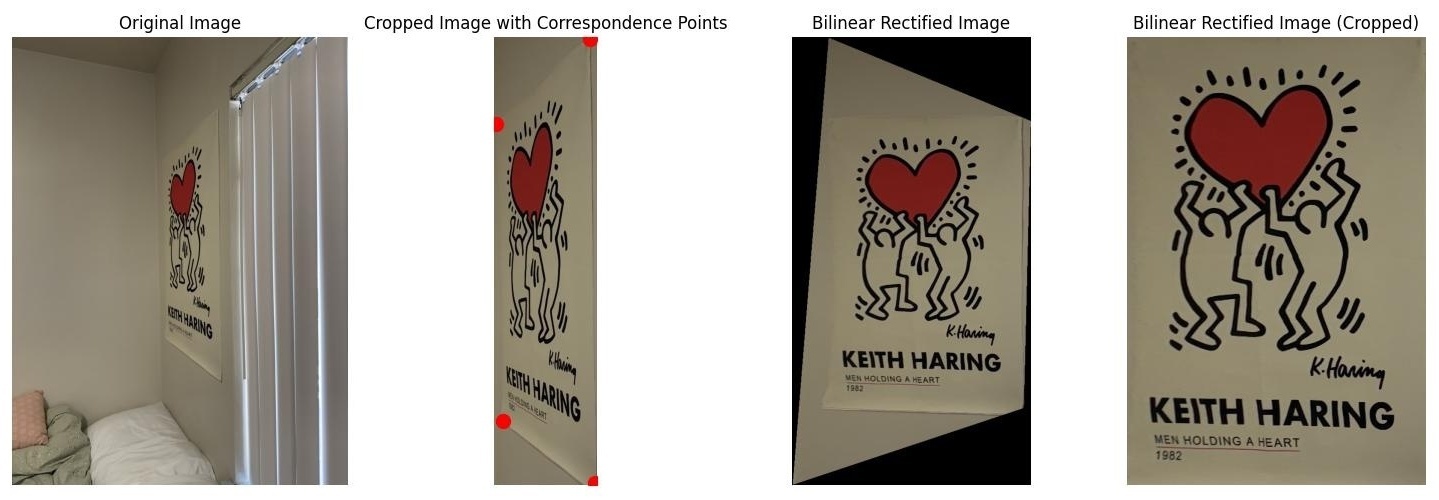
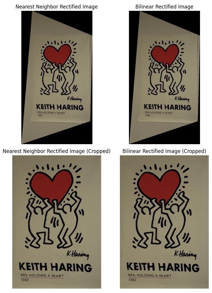
In the above comparison image, we can see that the bilinear interpolation results in a much smoother image than the nearest neighbor interpolation. If you look closely at the letters on the poster, you can see that the nearest neighbor interpolation results in a lot of blocky artifacts that are not present in the bilinear interpolation. However, the nearest neighbor interpolation is much faster than the bilinear interpolation. Timing the two functions on the Keith Haring poster: Bilinear time = 4.34 seconds, Nearest Neighbor time = 2.17 seconds. In my opinion, the bilinear interpolation is worth the slightly longer runtime because it results in a much smoother image. We will use bilinear interpolation for the rest of the project. For this rectification, I made a 400x600 rectangle to serve as the image_2 points for the homography calculation.

Full workflow of rectification of a tile from Portugal using bilinear interpolation. A 400x400 square was used as the image_2 points for the homography calculation.

Comparison of rectification results using nearest neighbor and bilinear interpolation of the same tile image.

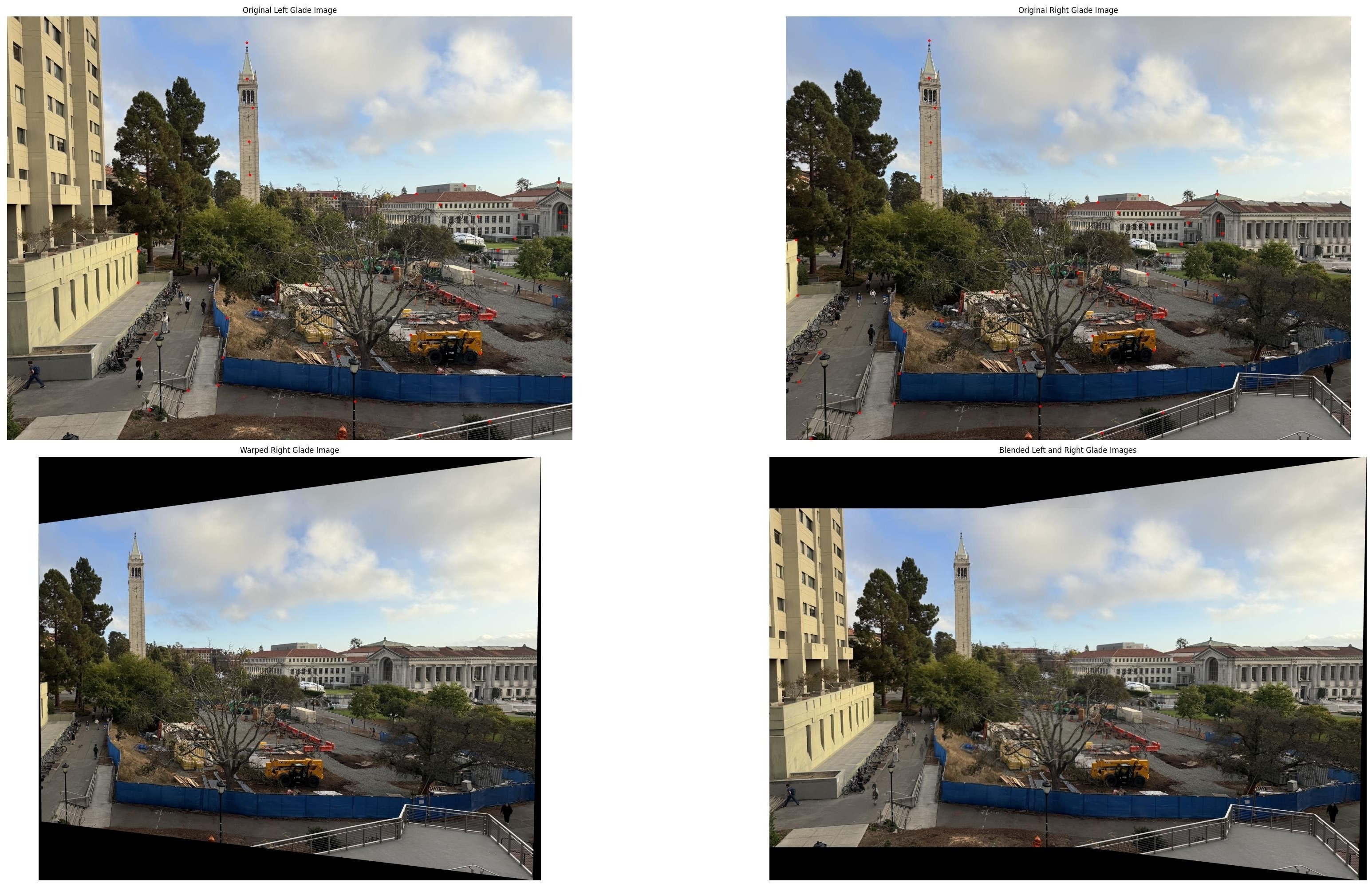
Part A.4: Blend Images into a Mosaic

With the ability to warp images, I can now create seamless mosaics by rectifying and blending multiple images. Instead of simple overwriting which creates harsh edge artifacts, I use weighted averaging and feathering techniques.

My approach involves picking one image as the reference image and warping the other images onto that reference image as the common projection plane by calculating the homography matrix between the other images and the reference image. We then warp the other images onto the reference image projection plane using the warp functions from earlier (all results below use bilinear interpolation) and then blend them using alpha masks. The alpha mask's values are determined by the method of blending used.

Alpha Masks and Weighted Blending

The key to seamless mosaicing is creating smooth transitions between overlapping images using alpha masks and weighted averaging. An alpha mask assigns each pixel a weight between 0 and 1, where 1 means "fully use this pixel" and 0 means "ignore this pixel completely."

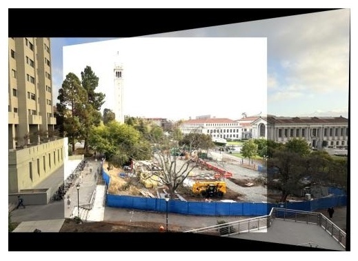
1. Simple 50/50 Blending (Uniform Weights)

The simplest blending approach treats all valid pixels equally:

# Create binary mask: 1 for valid pixels, 0 for black/invalid pixels
alpha = np.any(img > 0, axis=2).astype(float)

# Weighted averaging with uniform weights
final_pixel = (img1 * alpha1 + img2 * alpha2) / (alpha1 + alpha2)

This method simply checks if a pixel has any non-zero color values and assigns it weight 1 if valid, 0 if invalid (pure black). In overlapping regions, pixels are averaged 50/50. While simple, this creates visible seams because there's no gradual transition between images.

2. Linear Edge Falloff

To create smoother transitions, I implemented linear falloff where alpha values decrease linearly from the center toward the edges:

# Calculate distance to each edge
dist_up = y                    # distance from top edge
dist_down = h - y - 1         # distance from bottom edge  
dist_left = x                 # distance from left edge
dist_right = w - x - 1        # distance from right edge

# Find minimum distance to any edge
dist_to_closest_edge = np.minimum(
    np.minimum(dist_up, dist_down),
    np.minimum(dist_left, dist_right)
)

# Normalize to [0,1] and apply to valid pixels only
alpha = (dist_to_closest_edge / dist_to_closest_edge.max()) * mask

This creates alpha values that are highest at the center of each image and linearly decrease to 0 at the edges. The result is much smoother blending with gradual transitions, but the linear falloff can sometimes create visible gradients in the final mosaic.

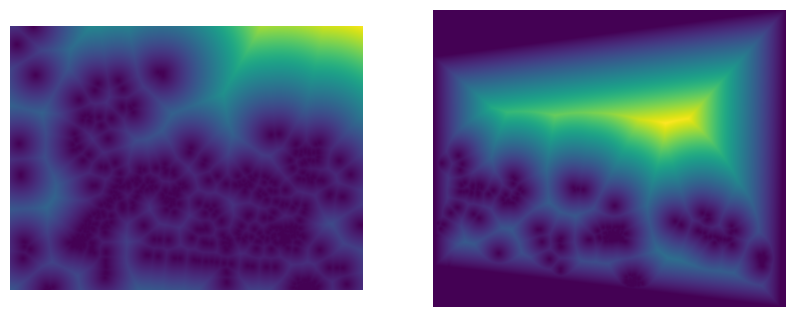
3. Distance Transform (scipy.ndimage.distance_transform_edt)

The Euclidean Distance Transform computes the distance from each valid pixel to the nearest invalid (black) pixel:

# Create binary mask of valid pixels
mask = np.any(image > 0, axis=2).astype(float)

# Compute distance to nearest black pixel
alpha = scipy.ndimage.distance_transform_edt(mask)

# Normalize and apply mask
alpha = (alpha / alpha.max()) * mask

This method works well when images have clean boundaries (black borders), creating natural feathering that follows the image shape. However, it fails when images contain legitimate black pixels in the content itself, as these are incorrectly treated as invalid regions, causing unwanted falloff in the middle of the image.

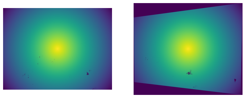
4. Centered Radial Falloff

To address the limitations of distance transform, I implemented a centered approach that creates radial falloff from the image center:

# Find image center
center_x, center_y = w / 2, h / 2

# Calculate distance from each pixel to center
y, x = np.ogrid[:h, :w]
dist_from_center = np.sqrt((x - center_x)**2 + (y - center_y)**2)

# Find maximum distance within valid region
max_dist = dist_from_center[mask > 0].max()

# Create radial falloff: 1 at center, 0 at furthest valid pixel
alpha = 1.0 - (dist_from_center / max_dist)
alpha = np.clip(alpha, 0, 1) * mask

This method creates smooth radial gradients that are independent of image content. The alpha values are highest at the image center and smoothly decrease toward the edges of the valid region. This approach works reliably regardless of image content and creates natural-looking blends.

5. Laplacian Stack Blending

For the most sophisticated blending, I implemented Laplacian stack blending, which performs frequency-domain blending to handle different spatial frequencies optimally. This technique, inspired by the classic Burt and Adelson paper, creates seamless blends by separating images into different frequency bands.

# 1. Create Gaussian stacks for both images and alpha mask
# 2. Create Laplacian stacks by taking differences between Gaussian levels
# 3. Blend each Laplacian level using the corresponding Gaussian alpha level
# 4. Reconstruct the final image by summing all blended Laplacian levels

The key insight is that different spatial frequencies should be blended at different scales. High-frequency details (fine textures, edges) are blended using sharp transitions, while low-frequency content (colors, gradual changes) uses smooth transitions.

Laplacian Stack Construction:

1. Gaussian Stack: Create multiple levels of increasingly blurred images
2. Laplacian Stack: Subtract consecutive Gaussian levels to isolate frequency bands
3. Alpha Gaussian Stack: Apply same Gaussian blurring to the alpha mask

# For each frequency level i:
# blended_laplacian[i] = laplacian_img1[i] * gaussian_alpha[i] + 
#                        laplacian_img2[i] * (1 - gaussian_alpha[i])
# 
# Final result = sum of all blended_laplacian levels + lowest_gaussian_level

This approach eliminates ghosting and seam artifacts more effectively than some of the other blending methods because it handles the transition of different frequency components separately. For all references to laplacian blending in the mosaic results below, I use linear alpha masks as the basis for the Laplacian blending, since linear falloff tends to deal with the edges of the images well. All laplacian stacks used below have 3 levels.

Weighted Averaging Process

All blending methods use the same weighted averaging formula:

# Accumulate weighted pixel values and weights
img_mosaic[y_min:y_max, x_min:x_max] += img_slice * alpha_slice[:, :, np.newaxis]
weight_map[y_min:y_max, x_min:x_max] += alpha_slice

# Normalize by total weights to get final pixel values
non_zero = weight_map > 1e-10
img_mosaic[non_zero] = img_mosaic[non_zero] / weight_map[non_zero, np.newaxis]

This ensures that overlapping regions are properly averaged according to their alpha weights, while non-overlapping regions retain their original pixel values. The small epsilon (1e-10) prevents division by zero in regions where no images contribute.

Mosaic Results

Blended mosaic of the glade images using weighted averaging and centered radial falloff.

Simple overlay of the glade images, without any blending.

Blended mosaic of the glade images using weighted averaging and all blending types.

Scipy distance-based alphas for the glade images. Since there are black points in the image itself, the alphas do not behave as expected.

Centered radial alphas for the glade images. Here you can see the points that are black in the original image, without it affecting the rest of the alpha values.

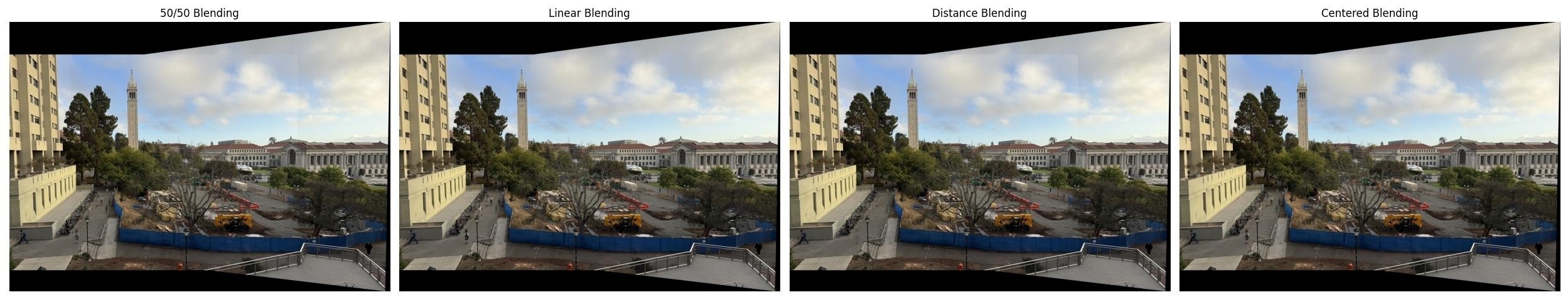
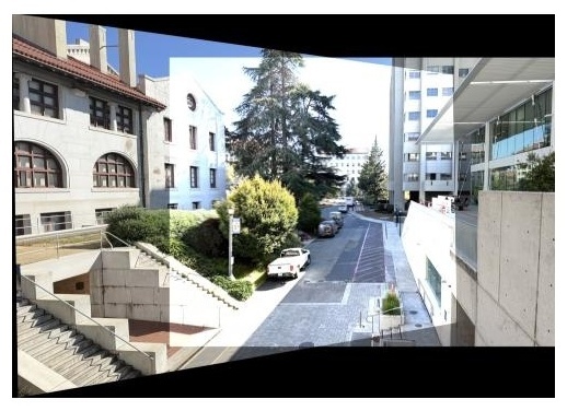
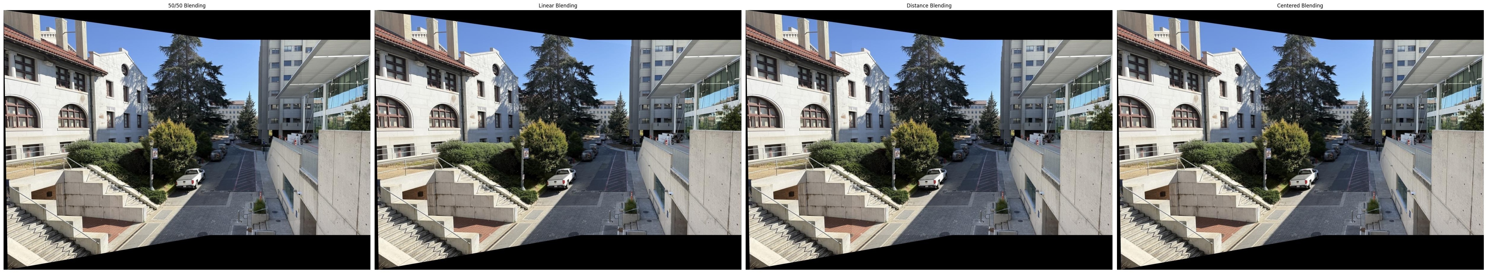
Versus the 50/50 blending, we can see that the centered radial falloff and the linear falloff look much better, without that harsh transition between the images in the top right corner, successfully removing the edge artifacts. We can still see some ghosting in the center image around the tree, suggesting that my center of projection may not have been perfectly fixed, or the points I selected may not have been perfect. The rest of the image areas where there is overlap look good though, such as the Campanile in the center of the image. The scipy distance-based alphas do not behave as expected since there are black points in the image itself, as you can see in the alpha mask images above. I also show the centered radial alphas, which perform better and remove the edge artifacts well.

Blended mosaic of the mining images using weighted averaging and centered radial falloff.

Simple overlay of the mining images, without any blending.

Blended mosaic of the mining images using weighted averaging and all blending types.

This image is remarkably good, with no edge artifacts and no ghosting besides a bit of blurring on the building in the far background. The blending looks great, with no harsh transitions between the images. This holds for all the blending types, which leads me to believe that my center of projection is pretty good, and the points I selected were good as well. There is a tiny bit of ghosting on the food vans in the center of the image, but it is not very noticeable.

Blended mosaic of the anchor house images using weighted averaging and centered radial falloff.

Simple overlay of the anchor house images, without any blending.

Blended mosaic of the anchor house images using weighted averaging and all blending types.

This blending is also great, with no edge artifacts and no ghosting besides people moving through the scene. As you can see, the edge artifacts shown in the simple overlay are removed by the blending. What is interesting about the different blending types here is how each version of blending deals with the person waiting for the crosswalk in this image. The 50/50 blending makes the person a ghost, while the linear falloff shows the person, and the laplacian of the linear falloff shows the person. The centered blending also shows the person, but they are slightly blurry. The distance transform blending gets rid of the person completely.

Part B: Feature Matching for Autostitching

In Part A, I manually selected correspondence points between images to compute homographies. This is tedious and error-prone. In Part B, I implement an automated feature detection and matching system that can automatically find correspondences between images. This allows for fully automatic image mosaicing without any manual intervention. I follow the approach outlined in the paper "Multi-Image Matching using Multi-Scale Oriented Patches" by Brown et al., with some simplifications as specified in the project instructions.

Part B.1: Harris Corner Detection

The first step in automatic feature matching is detecting interest points, or "corners", in both images. I use the Harris Corner Detector to find corners, which are points where image gradients change significantly in multiple directions. These corners are distinctive features that are likely to be recognizable in different views of the same scene.

Preprocessing: Before applying Harris corner detection, I convert the RGB images to grayscale using skimage.color.rgb2gray. Harris corner detection operates on intensity values, analyzing how brightness changes in different directions. Converting to grayscale produces a single-channel intensity image that captures the luminance information needed for gradient computation, regardless of color variations.

Algorithm Overview

The Harris corner detection algorithm works by analyzing how image gradients change in different directions at each pixel. A true corner should have significant gradient changes in multiple directions (unlike an edge, which only has gradients in one direction, or a flat region with no gradients). The algorithm produces a corner response matrix where each pixel's value indicates its corner strength.

Harris Corner Detection Process:

FUNCTION get_harris_corners(image, parameters):
    
    1. COMPUTE corner strength matrix:
       - For each pixel, compute image gradients in x and y directions
       - Build structure tensor from gradient products (Ix², Iy², IxIy)
       - Apply Gaussian weighting to structure tensor
       - Compute corner strength: R = det(M) / trace(M)
       - Result: H matrix where H[y,x] = corner strength at pixel (x,y)
    
    2. FIND local maxima in response matrix:
       - Search for peaks in H that are local maxima within min_distance radius
       - Apply threshold to keep only corners stronger than threshold_rel * max(H)
       - Result: List of (y, x) coordinates of potential corners
    
    3. FILTER corners near image boundaries:
       - Remove any corners within edge_discard pixels of image borders
       - This ensures we can safely extract feature descriptors later
       - Result: (2, N) array of corner coordinates, [y-coords; x-coords]
    
    RETURN corner_strength_matrix, corner_coordinates

The key insight is that the Harris response combines information from both eigenvalues of the structure tensor. At a corner, both eigenvalues are large (gradients in multiple directions). At an edge, only one eigenvalue is large. In flat regions, both are small. The response formula efficiently captures this without computing eigenvalues explicitly.

Mathematical Formulation:

The Harris corner response is computed as:

where the structure tensor \(M\) at each pixel is:

The determinant and trace are related to the eigenvalues \(\lambda_1, \lambda_2\) of \(M\):

Therefore, the corner response can be expressed as:

The response \(R\) allows us to classify image regions:

• Corner: Both \(\lambda_1\) and \(\lambda_2\) are large → \(R\) is large
• Edge: One eigenvalue large, i.e. (\(\lambda_1\)), one small (\(\lambda_2\)) → \(R \approx 2\lambda_2\) (small)
• Flat region: Both eigenvalues small → \(R\) is small

The key insight is that for a corner, the product \(\lambda_1 \lambda_2\) is large (both eigenvalues are large), while for an edge, even if one eigenvalue is large, the product divided by the sum is dominated by the smaller eigenvalue, making \(R\) small.

Key Parameters:

• sigma: Controls the scale of the Gaussian smoothing applied before computing gradients. I use sigma=1 for single-scale detection as suggested in the project starter code.
• min_distance: Minimum distance between detected corners in pixels. This suppresses nearby corners to avoid clustering. I experimented with values of 10, 25, and 50 pixels.
• threshold_rel: Relative threshold for corner strength (as a fraction of the maximum response). Only corners stronger than threshold_rel * max(h) are kept. I tested values of 0.01, 0.05, and 0.1.
• edge_discard: Pixels to discard from image borders (minimum 20 pixels) to ensure feature descriptors can be safely extracted without going out of bounds.

Harris corners detected on the left anchor house image using min_distance=50, threshold_rel=0.01.

Harris corners detected on the left Haste street image using min_distance=50, threshold_rel=0.01.

Parameter Exploration

To understand how parameters affect corner detection, I tested different values:

Effect of min_distance parameter on anchor house image: 10, 25, and 50 pixels. Larger values spread corners more evenly across the image.

Effect of min_distance parameter on Haste street image: 10, 25, and 50 pixels.

Effect of threshold_rel parameter on anchor house image: 0.01, 0.05, and 0.1. Higher thresholds select only the strongest corners, reducing the total count. Min_distance=50.

Effect of threshold_rel parameter on Haste street image: 0.01, 0.05, and 0.1. Min_distance=50.

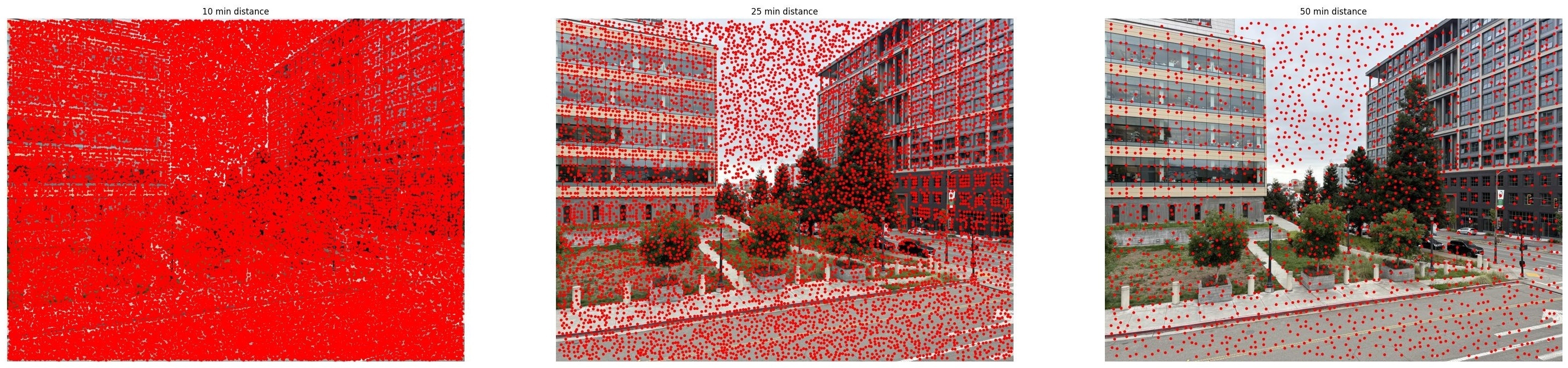
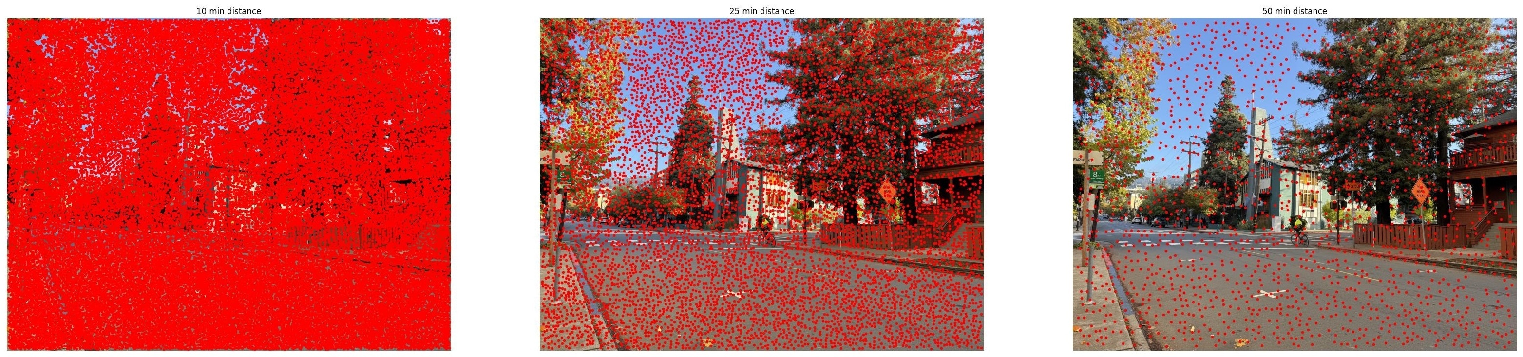
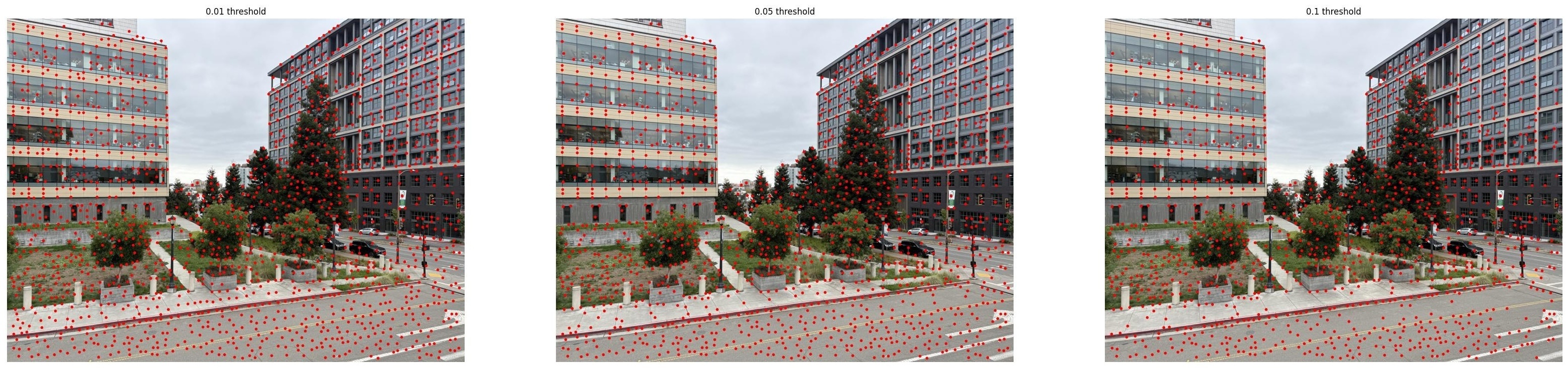
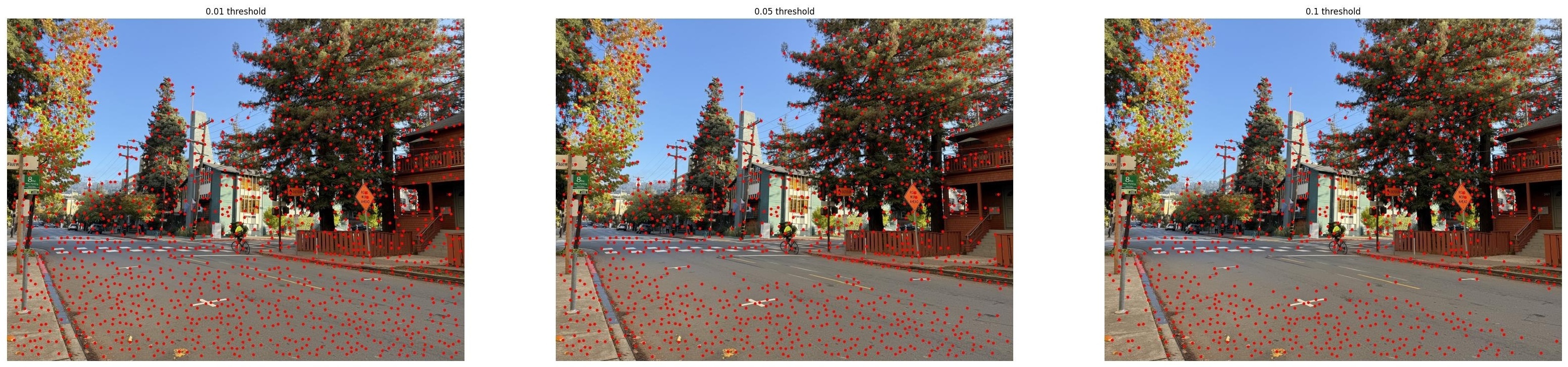
The min_distance parameter controls spatial distribution: smaller values allow corners to cluster together, while larger values enforce more even spacing. The threshold_rel parameter controls quality: lower values include weaker corners, while higher values keep only the strongest features. For the next part of the project (through part B.3), I use min_distance=10 to detect many corners, then apply Adaptive Non-Maximal Suppression (ANMS) to select the best distributed subset.

Adaptive Non-Maximal Suppression (ANMS)

Raw Harris corner detection often produces thousands of corners, many clustered in high-texture regions. Adaptive Non-Maximal Suppression solves this by selecting a subset of corners that are well-distributed across the image while prioritizing strong corners. The algorithm comes from Section 3 of the Brown et al. paper.

ANMS Algorithm:

For each corner \(i\), we compute its suppression radius \(r_i\): the distance to the nearest corner that is significantly stronger. Formally:

where \(f(\mathbf{x})\) is the Harris corner strength, and \(c_{\text{robust}} = 0.9\) is a robustness constant. Corners with larger suppression radii are more "isolated" in their strength and are preferred.

The Logic Behind ANMS:

The fundamental idea is that a good feature point should be locally the strongest in its neighborhood. If a corner has many stronger corners nearby, it's redundant. But if the nearest stronger corner is far away, this corner is providing unique information about that region of the image.

FUNCTION adaptive_non_maximal_suppression(corners, strengths, num_to_select):

    1. INITIALIZE suppression radius for each corner to infinity
    
    2. COMPUTE pairwise distances between all corners:
       - Create distance matrix D where D[i,j] = distance from corner i to corner j
       - This can be done efficiently: ||xi - xj||² = ||xi||² + ||xj||² - 2⟨xi, xj⟩
    
    3. FOR each corner i:
         a. FIND all corners j that are significantly stronger:
            - stronger_mask[j] = True if strength[j] > strength[i] / c_robust
            - The division by c_robust makes the test slightly lenient
         
         b. IF any stronger corners exist:
            - suppression_radius[i] = minimum distance to any stronger corner
         ELSE:
            - suppression_radius[i] = infinity (this is the strongest corner)
    
    4. SORT corners by suppression radius (largest first)
       - Corners with large radii are "isolated peaks" in the strength landscape
       - These are the most informative features
    
    5. SELECT top num_to_select corners with largest suppression radii
    
    RETURN selected_corners, their_indices, all_suppression_radii

Why this works: Consider two scenarios. In a high-texture region (like a building facade), many corners will be detected close together. Most will have small suppression radii because there are stronger corners nearby. Only the very strongest corners in that region will have larger radii. In contrast, a moderately strong corner in an otherwise smooth region might have a very large suppression radius because the nearest stronger corner is far away. ANMS balances these cases, selecting corners that are both strong AND well-distributed.

The robustness constant \(c_{\text{robust}} = 0.9\) adds tolerance: we don't require neighbors to be strictly stronger, just stronger by a factor of 0.9. This prevents numerical instabilities when corners have very similar strengths.

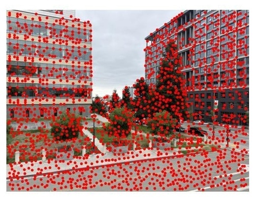
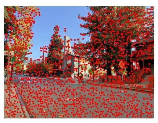
ANMS vs. Simple Thresholding

The comparison below shows why ANMS is superior to simply selecting the 500 strongest Harris corners:

Top row: 500 strongest Harris corners (left) vs. ANMS-selected corners (right) for anchor house image. Bottom row: Same comparison with threshold_rel=0.01. ANMS produces much better spatial distribution across the entire image, while strongest corners cluster in high-texture regions like the building facade.

Comparison of 500 strongest Harris corners (left) vs. ANMS-selected corners (right) for the Haste street image. ANMS provides better spatial distribution across street signs, buildings, and foliage.

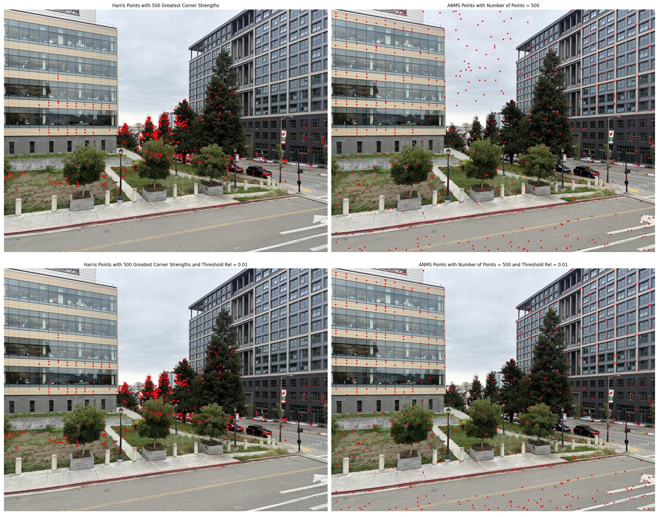
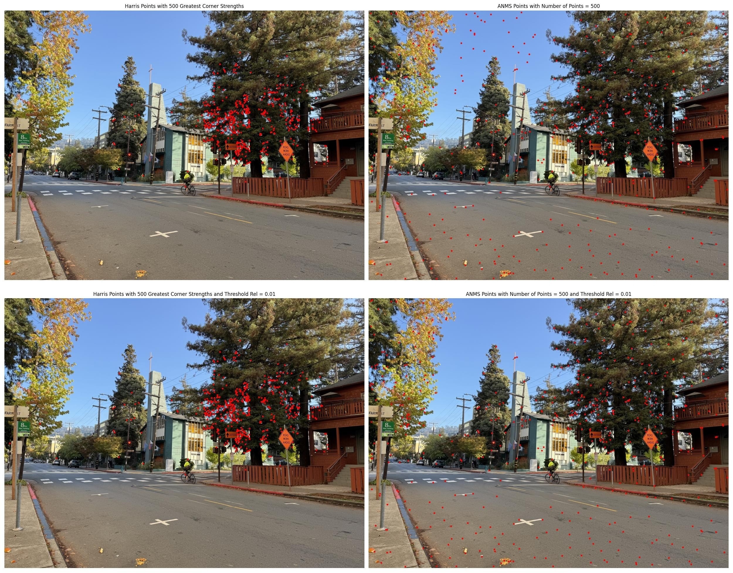
The ANMS-selected corners are much better distributed across the images, including diverse regions like sky, trees, building facades, and street infrastructure. Simple strength-based selection produces heavy clustering in high-texture regions, leaving other areas underrepresented. This balanced distribution is crucial for robust homography estimation.

Part B.2: Feature Descriptor Extraction

After detecting corner locations, I need to create feature descriptors: compact representations that capture the local appearance around each corner. These descriptors enable matching corners between images even when viewpoints change. I implement the approach from Section 4 of the Brown et al. paper, using axis-aligned 8×8 descriptors sampled from 40×40 pixel windows.

Feature Descriptor Extraction Pipeline

A feature descriptor must compactly represent the local appearance around a corner point in a way that's robust to variations in viewpoint, lighting, and small geometric distortions. The challenge is balancing distinctiveness (descriptors from different locations should look different) with repeatability (the same physical point in different images should produce similar descriptors).

The Four-Step Extraction Process:

1. Gaussian Blur: Smooth the image with \(\sigma=1.5\) to create a blurred descriptor that's less sensitive to small pixel-level noise and aliasing
2. Sample 40×40 Window: Define a large window centered on the corner point to capture sufficient context
3. Subsample to 8×8: Sample 8×8 points evenly spaced within the 40×40 window (every 5 pixels), using bilinear interpolation for subpixel accuracy
4. Bias-Gain Normalize: Normalize the descriptor to zero mean and unit variance to achieve invariance to brightness and contrast changes

FUNCTION get_feature_descriptors(grayscale_image, corner_locations):

    CONSTANTS:
        window_size = 40 pixels        # Large window for context
        descriptor_size = 8 × 8 = 64   # Compact representation
        spacing = 40 / 8 = 5 pixels    # Sample every 5 pixels
        blur_sigma = 1.5               # Smoothing parameter
    
    1. PREPROCESS image:
       - Apply Gaussian blur with σ = 1.5 to entire image
       - This creates "nice big blurred descriptors" as mentioned in the paper
       - Reduces high-frequency noise, makes descriptors more robust
    
    2. FOR each corner location (x_center, y_center):
       
       a. CHECK boundary conditions:
          - If window extends outside image (±20 pixels from corner)
          - Mark this descriptor as invalid and skip
          - Ensures we only extract complete descriptors
       
       b. CREATE sampling grid:
          - Start at (x_center - 20, y_center - 20)  [top-left of window]
          - Sample 8 points in each direction with spacing = 5
          - Sampling positions: -17.5, -12.5, -7.5, ..., +17.5 from center
          - These are at the CENTERS of 5×5 pixel blocks
       
       c. EXTRACT descriptor values via bilinear interpolation:
          - For each of 64 sample positions (y, x):
          - Find four surrounding pixels: (⌊x⌋, ⌊y⌋), (⌈x⌉, ⌊y⌋), etc.
          - Compute weights based on fractional parts
          - Interpolated value = weighted average of four pixels
          - This provides subpixel accuracy
       
       d. NORMALIZE descriptor (bias-gain normalization):
          - Compute μ = mean of 64 values
          - Compute σ = standard deviation of 64 values  
          - Normalized descriptor = (values - μ) / (σ + ε)
          - Result: zero mean, unit variance
          - Invariant to affine intensity changes: I' = aI + b
    
    3. RETURN descriptors and validity flags

Why These Design Choices?

Each design decision addresses a specific challenge in feature matching:

• 40×40 window → 8×8 descriptor: The large window captures enough context to be distinctive (can distinguish between different image regions), while downsampling to 8×8 keeps the descriptor compact (only 64 dimensions) and reduces noise. The paper emphasizes sampling from a "nice big blurred descriptor" rather than directly extracting an 8×8 patch. This 5:1 downsampling ratio provides natural smoothing.
• Bilinear interpolation: Since our sampling grid might not align perfectly with pixel boundaries, we interpolate. Consider sampling at position (10.5, 10.5) - we take a weighted average of pixels (10,10), (11,10), (10,11), and (11,11) with weights based on distance. This provides subpixel accuracy and makes descriptors less sensitive to small translations or rotations.
• Gaussian blur (σ=1.5) before sampling: This is crucial for robustness. Without blur, tiny pixel-level noise or aliasing artifacts would contaminate the descriptor. With blur, we're effectively looking at "blurred patches" which are more stable across different images of the same scene. The σ=1.5 value provides moderate smoothing without losing too much detail.
• Bias-gain normalization: This makes descriptors invariant to affine intensity changes. If image 2 is brighter than image 1 (\(I_2 = aI_1 + b\)), the normalized descriptors will still match because we remove the mean (eliminates \(b\)) and divide by standard deviation (eliminates \(a\)). Mathematically: $$\text{descriptor} = \frac{\text{values} - \mu}{\sigma + \epsilon}$$ The epsilon (typically \(10^{-10}\)) prevents division by zero in constant-valued patches.
• Boundary checking: We need a full 40×40 window around each corner. Corners within 20 pixels of image edges can't provide complete descriptors, so we mark them invalid rather than using partial or zero-padded windows which would produce unreliable descriptors.

A key insight: We don't store raw pixel values; we store normalized intensity patterns. Two image patches that have the same "texture" but different brightnesses will produce nearly identical descriptors. This is why the method works across images taken with different exposures or lighting conditions.

Left: Anchor house image with two ANMS corner points highlighted (red and magenta). Middle/Right: Their corresponding 8×8 feature descriptors shown as grayscale patches. Each descriptor captures the local texture pattern around its corner after bias-gain normalization.

Left: Haste street image with three ANMS corner points highlighted (blue, cyan, and magenta). Middle/Right: Their corresponding 8×8 feature descriptors shown as grayscale patches. The blue point captures texture from the bike wheel, the cyan point shows patterns from the street light, and the magenta point captures texture from the tree branches.

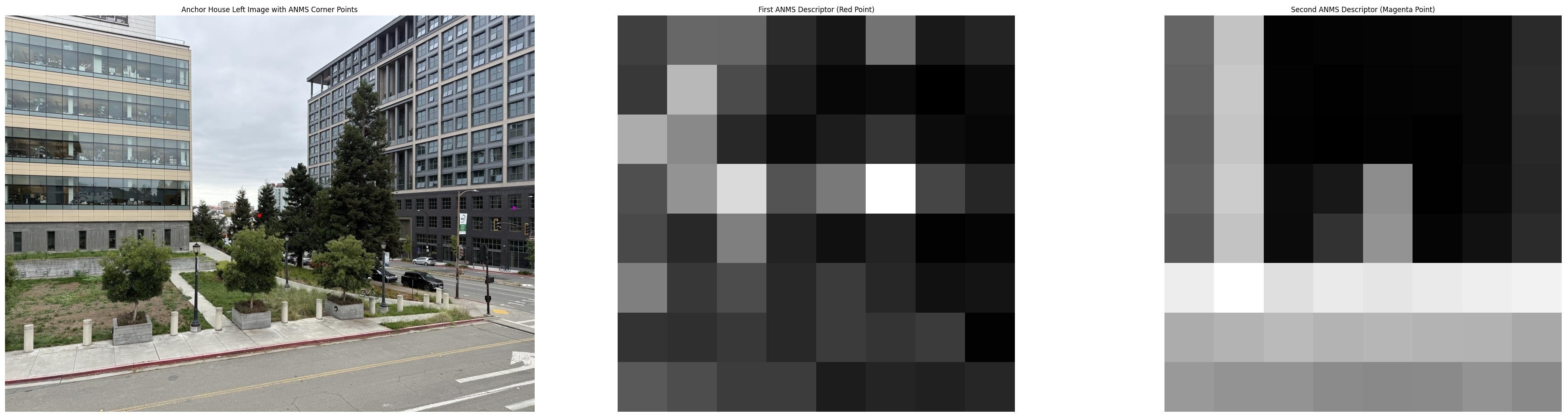
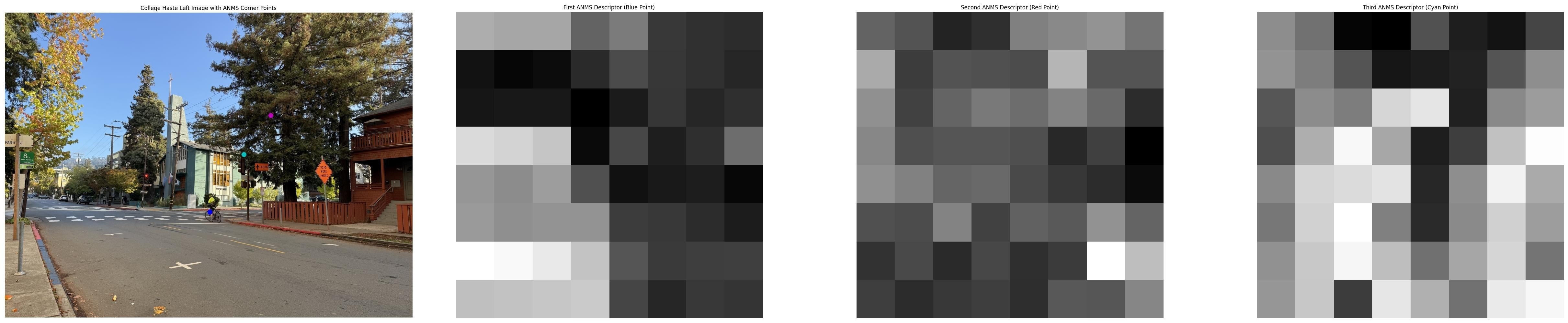
The visualized descriptors show how different image regions produce distinct patterns. In the anchor house example, the red point's descriptor captures interesting texture pattern from the tree branches, while the magenta point's descriptor shows straight lines of the building window. In the Haste street example, descriptors capture varied textures from the bike wheel, the street light, and the tree branches. These distinctive signatures enable reliable matching across images.

Part B.3: Feature Matching

With feature descriptors extracted from both images, I now need to find corresponding features. I implement mutual nearest neighbor matching with Lowe's ratio test to create reliable matches between image pairs.

Feature Matching Algorithm

Given descriptors from two images, how do we decide which pairs correspond to the same physical point? The naive approach—just match each descriptor to its nearest neighbor—produces many false matches because similar-looking textures (like windows, bricks, or leaves) create ambiguous correspondences. I use two complementary strategies to ensure reliable matching:

Strategy 1: Lowe's Ratio Test

The Problem: Repetitive textures create ambiguous matches. If descriptor A looks very similar to both descriptor B and descriptor C, we can't confidently say which is the correct match.

Lowe's Solution: A match is only reliable if the nearest neighbor is significantly closer than the second-nearest neighbor. Formally, accept a match only if:

With threshold = 0.8, we require the best match to be at least 25% closer than the second-best match. If the ratio is close to 1.0, the match is ambiguous and we reject it. If the ratio is small (say, 0.5), there's a clear winner and we accept it.

Strategy 2: Matching Direction - One-Directional vs. Two-Directional

After applying Lowe's ratio test, we still need to decide how to establish correspondences between descriptors. I implement both one-directional matching and two-directional (mutual) matching, each with different trade-offs:

One-Directional Matching

How it works: For each descriptor in image 1, find its nearest neighbor in image 2 (subject to ratio test). This creates a set of matches from image 1 → image 2.

Trade-offs: This approach produces more matches but with potentially lower quality. Multiple descriptors in image 1 can all match to the same descriptor in image 2 (many-to-one), and there's no requirement for agreement in the reverse direction. Some matches may be asymmetric—descriptor A in image 1 matches to B in image 2, but B's best match is actually to some other descriptor C in image 1.

Two-Directional (Mutual) Matching

How it works: Require bidirectional agreement. Only accept (A, B) as a match if:

• A's nearest neighbor in image 2 is B (passes ratio test), AND
• B's nearest neighbor in image 1 is A (passes ratio test)

Trade-offs: This symmetry requirement is very powerful—false matches rarely satisfy both directions because accidental similarity is unlikely to be reciprocal. Two-directional matching produces fewer but higher-quality matches. Each match is a true mutual nearest neighbor, eliminating most asymmetric correspondences and many-to-one mappings.

When to Use Which Method

For this section (B.3), I use two-directional matching to demonstrate clean, high-quality correspondences without downstream robust estimation. The mutual agreement ensures that the visualized matches are highly reliable.

However, when using RANSAC (section B.4), I switch to one-directional matching. Why? RANSAC is specifically designed to handle outliers robustly—it will automatically detect and discard incorrect matches during homography estimation. By using one-directional matching, we feed more candidate matches into RANSAC, giving it a larger pool of correspondences to work with. RANSAC's iterative sampling and consensus mechanism will prune the outliers anyway, so we prioritize quantity over initial quality to improve the chances of finding good inlier sets. This trade-off makes sense because RANSAC's strength is precisely its ability to handle contaminated data.

FUNCTION match_descriptors_two_sided(descriptors_img1, descriptors_img2, ratio_threshold):

    1. COMPUTE pairwise distances:
       - Flatten each 8×8 descriptor to 64-dimensional vector
       - Compute distance matrix D where D[i,j] = ||desc1[i] - desc2[j]||
       - Use Euclidean distance in 64-dimensional space
       - This can be vectorized for efficiency: ||a-b||² = ||a||² + ||b||² - 2⟨a,b⟩
    
    2. FIND left-to-right candidate matches (image 1 → image 2):
       - For each descriptor i in image 1:
         a. Find two nearest neighbors in image 2:
            - nn1 = descriptor with smallest distance to i
            - nn2 = descriptor with second-smallest distance to i
         
         b. Apply Lowe's ratio test:
            - ratio = distance(i, nn1) / distance(i, nn2)
            - IF ratio < threshold (typically 0.8):
                - Store: left_to_right_matches[i] = nn1
                - This is a candidate match
            - ELSE:
                - Reject (too ambiguous)
    
    3. FIND right-to-left candidate matches (image 2 → image 1):
       - Same process in reverse direction
       - For each descriptor j in image 2:
         - Find its nearest and second-nearest neighbors in image 1
         - Apply ratio test
         - Store: right_to_left_matches[j] = nn1
    
    4. KEEP only mutual matches (bidirectional agreement):
       - For each candidate match (i → j) from step 2:
         - CHECK if j → i exists in step 3
         - IF yes: this is a mutual match, keep it
         - IF no: one-way match only, discard it
       
       - Result: Each matched pair satisfies BOTH:
         1. i's best match is j (with good ratio)
         2. j's best match is i (with good ratio)
    
    RETURN list of matched pairs (i, j)

FUNCTION match_descriptors_one_sided(descriptors_img1, descriptors_img2, ratio_threshold):

    1. COMPUTE pairwise distances:
       - Flatten each 8×8 descriptor to 64-dimensional vector
       - Compute distance matrix D where D[i,j] = ||desc1[i] - desc2[j]||
       - Use Euclidean distance in 64-dimensional space
    
    2. FIND left-to-right matches (image 1 → image 2):
       - For each descriptor i in image 1:
         a. Find two nearest neighbors in image 2:
            - nn1 = descriptor with smallest distance to i
            - nn2 = descriptor with second-smallest distance to i
         
         b. Apply Lowe's ratio test:
            - ratio = distance(i, nn1) / distance(i, nn2)
            - IF ratio < threshold (typically 0.8):
                - Accept match: (i, nn1)
            - ELSE:
                - Reject (too ambiguous)
    
    3. RETURN all accepted matches
       - Note: No bidirectional check, so multiple i's can match same j
       - This produces more matches than two-sided matching

Why This Works:

Lowe's ratio test eliminates ambiguous matches. In repetitive regions (brick walls, windows), many descriptors look similar, so the ratio approaches 1.0 and we reject them. In distinctive regions (unique corners, irregular textures), the nearest neighbor is much closer than alternatives, ratio is small, and we accept them.

Two-directional (mutual) matching eliminates asymmetric errors. Consider a textured region in image 1 that's occluded in image 2. Descriptors from that region might match to something in image 2 (one-way), but those image 2 descriptors have better matches elsewhere, so the match won't be mutual. Only true correspondences—the same physical point visible in both images—consistently produce mutual matches.

One-directional matching is more permissive, accepting any forward match that passes the ratio test. While this introduces more false positives, it provides more candidates for downstream robust estimation algorithms like RANSAC to work with.

Combined effect: For the demonstrations in this section, the ratio test + two-directional matching work together beautifully. Ratio test removes ambiguous matches (low-confidence), and mutual nearest neighbors removes incorrect matches (mismatches). What remains is a high-quality set of correspondences. For RANSAC-based workflows, using one-directional matching provides a larger candidate pool while RANSAC handles outlier rejection.

Effect of Ratio Threshold

The ratio threshold controls the trade-off between match quantity and quality. The following results use two-directional matching to demonstrate clean correspondences:

Anchor house (two-directional matching): Top row shows all ANMS corners detected (blue points). Middle row: Matches with ratio_threshold=1.0 (accepts all matches). Third row: Matches with ratio_threshold=0.8 (balanced). Bottom row: Matches with ratio_threshold=0.6 (very strict). Lower thresholds produce fewer but more reliable matches.

Haste street (two-directional matching): Top row shows all ANMS corners detected (blue points). Middle row: Matches with ratio_threshold=1.0. Third row: Matches with ratio_threshold=0.8. Bottom row: Matches with ratio_threshold=0.6. The Haste street scene has rich texture from buildings and foliage, producing many reliable matches even with stricter thresholds.

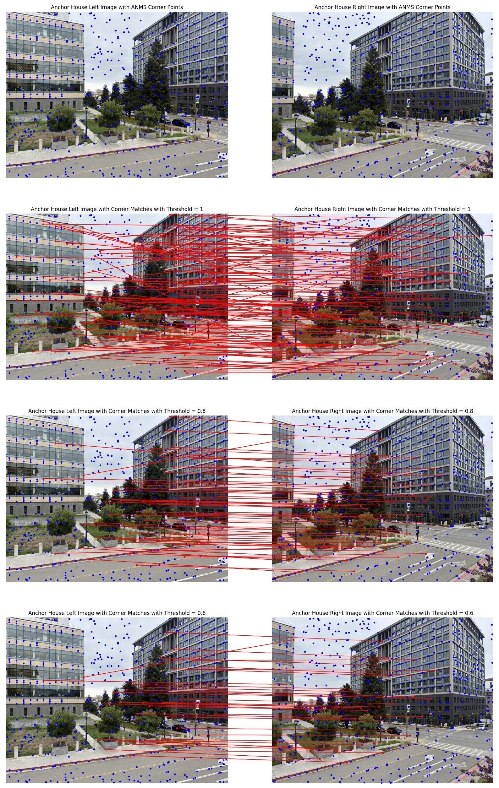
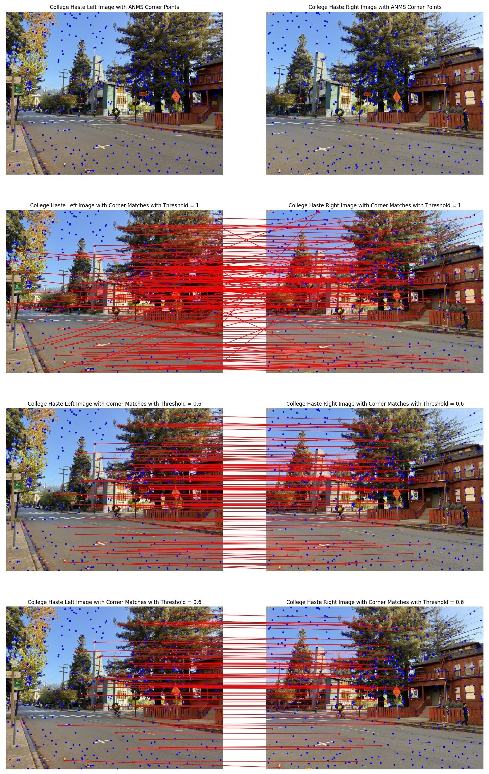
With ratio_threshold=1.0, we accept nearly all nearest neighbor matches, including many false positives from ambiguous or repetitive textures. With ratio_threshold=0.6, we get very high-quality matches but fewer overall. The default ratio_threshold=0.8 provides a good balance: enough matches for robust homography estimation while filtering most false positives.

Part B.4: RANSAC for Robust Homography Estimation

Even with careful feature matching, some incorrect correspondences (outliers) inevitably remain. RANSAC (RANdom SAmple Consensus) is a robust estimation technique that can compute an accurate homography even when a significant fraction of matches are wrong. I implement 4-point RANSAC as described in class.

Note on matching strategy: For all RANSAC-based results in this section, I use one-directional matching instead of the two-directional matching shown in section B.3. As explained earlier, one-directional matching provides more candidate correspondences for RANSAC to work with, and RANSAC's robust estimation naturally filters out the additional outliers. This trade-off—more matches with more outliers, but handled by RANSAC—produces better final results than starting with fewer, higher-quality matches.

RANSAC Algorithm Overview

RANSAC (RANdom SAmple Consensus) is an elegant solution to a fundamental problem: how do we fit a model when some of our data points are completely wrong? Traditional least-squares fitting assumes all points have small errors, but with feature matching, some correspondences are outliers: completely incorrect matches that don't satisfy any geometric relationship.

The Core Insight:

Instead of trying to fit all points at once (which outliers would corrupt), RANSAC repeatedly fits models to small random subsets and asks: "How many of the other points agree with this model?" The model that explains the most data points is likely the correct one. Outliers rarely agree with any model, so they're automatically excluded.

RANSAC for Homography Estimation:

FUNCTION ransac_homography(matches, points_img1, points_img2, epsilon, num_iterations):

    INITIALIZE:
        best_H = None
        best_inliers = []
        best_num_inliers = 0
    
    REPEAT num_iterations times:
        
        1. RANDOM SAMPLE:
           - Randomly select 4 matched point pairs
           - Each pair (p1[i], p2[i]) is a correspondence
           - 4 is the minimum needed to solve for a homography (8 DOF)
        
        2. COMPUTE HOMOGRAPHY:
           - Solve for H using these 4 pairs (as in Part A)
           - This gives us a candidate homography matrix
        
        3. COUNT INLIERS:
           - For EVERY match (not just the 4 we sampled):
             a. Transform point from img1 using H: p2_predicted = H * p1
             b. Compute reprojection error: error = ||p2_predicted - p2_actual||
             c. If error < epsilon pixels: this match is an inlier
           
           - Total inliers = number of matches that agree with H
        
        4. UPDATE BEST:
           - If num_inliers > best_num_inliers:
             - Save this H as best_H
             - Save which matches are inliers
             - Update best_num_inliers
    
    5. REFINEMENT (after all iterations):
       - We now have a set of inlier matches (likely correct)
       - Recompute H using ALL inliers (not just 4)
       - This improves accuracy since we're using more data
       - Least-squares with inliers only is much better than with outliers
    
    RETURN best_H, inlier_mask, num_inliers

Computing Inliers (The Agreement Test):

For a candidate homography \(H\), we test each match \((p_1, p_2)\) by computing the reprojection error:

1. Transform \(p_1\) from image 1 to image 2 coordinates: \(p_2' = H p_1\) (in homogeneous coordinates)
2. Measure distance between predicted position \(p_2'\) and actual position \(p_2\): $$\text{error} = \|p_2' - p_2\|$$
3. If error < \(\epsilon\) (I use \(\epsilon = 3\) pixels), count this as an inlier

A match is an inlier if it's consistent with the geometric transformation \(H\). The threshold \(\epsilon = 3\) pixels allows for small errors from feature detection imprecision or interplolation, but rejects matches that are geometrically impossible under that homography.

Why RANSAC Works

The probability that all 4 randomly selected matches are inliers (and thus produce a good homography) is:

The probability of getting at least one good sample in \(n\) iterations is: \(1 - (1 - p^4)^n\), where \(p\) is the inlier ratio. Even with challenging scenes where only 10-20% of matches are inliers, running 100,000 iterations gives us excellent success probability:

• 10% inliers: \(1 - (1 - 0.1^4)^{100000} \approx 0.99995\) (99.995% success rate)
• 20% inliers: \(1 - (1 - 0.2^4)^{100000} \approx 1.0\) (essentially 100% success rate)

Each good sample produces a candidate homography, and we keep the one with the most agreement (inliers). This is why RANSAC is so powerful—even with a majority of outliers, sufficient iterations ensure we find the correct geometric transformation.

Complete Automatic Stitching Pipeline

Now I can combine all the components into a complete system that takes two images and produces a stitched mosaic with zero manual intervention:

FUNCTION automatic_image_stitching(image1, image2):

    1. PREPROCESSING:
       - Convert both images to grayscale for feature detection
       - Color information isn't useful for finding corners
    
    2. HARRIS CORNER DETECTION:
       - Detect corners in both images
       - Parameters: min_distance = 15, threshold_rel = 0.01
       - Results: Thousands of potential corner points per image
    
    3. ADAPTIVE NON-MAXIMAL SUPPRESSION:
       - Select best 1000 corners from each image
       - These are well-distributed across the image
       - Avoids clustering in high-texture regions
    
    4. FEATURE DESCRIPTOR EXTRACTION:
       - Extract 8×8 descriptor for each corner (from 40×40 window)
       - Apply Gaussian blur (σ = 1.8) and bias-gain normalization
       - Filter out invalid descriptors (too close to image boundaries)
       - Results: ~1000 valid descriptors per image
    
    5. FEATURE MATCHING:
       - Match descriptors using mutual NN + Lowe's ratio test (threshold = 0.8)
       - Results: Typically 100-200 matched pairs
       - Some are correct correspondences, some are outliers
    
    6. RANSAC FOR ROBUST HOMOGRAPHY:
       - Run 100,000 RANSAC iterations with ε = 3 pixels
       - Finds best homography that explains the most matches
       - Results: ~50-100 inliers (correct matches), outliers rejected
    
    7. REFINEMENT:
       - Recompute homography using all inlier matches
       - This gives more accurate H than using just 4 random points
    
    8. IMAGE WARPING:
       - Warp one image to align with the other using H
       - Use bilinear interpolation for smooth results
       - Compute output canvas size to fit entire warped image
    
    9. ALPHA BLENDING:
       - Blend warped and reference images using alpha masks
       - Use some simple falloff for smooth transitions between images (linear, distance, centered, or laplacian blending)
       - Results: mosaic with minimal visible seams
    
    RETURN final_mosaic

The power of this pipeline is that each stage progressively filters and refines the data:

1. Harris → Many candidate features (quantity)
2. ANMS → Well-distributed subset (spatial balance)
3. Descriptors → Distinctive representations (quality)
4. Matching → Likely correspondences (pruning)
5. RANSAC → Geometrically consistent inliers (robustness)

By the time we reach homography estimation, we've filtered 20,000 raw corners down to ~50-100 high-confidence inliers. This multi-stage filtering is what makes automatic stitching reliable in practice.

Results: Manual vs. Automatic Stitching

Now I can compare the quality of manual stitching (Part A, with hand-selected correspondences) versus automatic stitching (Part B, with detected and matched features). For each of the following, I tried different parameters for the automatic stitching pipeline to improve the results. I ended up settling on the following parameters: min_distance=15, threshold_rel=0.01, sigma=1.8, and ratio_threshold=0.8.

Anchor House Comparison

Automatic stitching result using the full RANSAC pipeline versus manual stitching.

The automatic result doesn't align the images as well as the manual stitching. There are some slight artifacts in the image, such as the top of the anchor house being slightly off. I think this is because the automatic stitching may struggle with the repetitive texture of the anchor house building as well as the building on the left. There isn't much overlap between the images when it comes to these buildings as well, so the good corners being chosen might not mostly be in the overlap of the images. There is also a decent amount of sky, which has minimal texture, making it difficult for the automatic stitching to find good feature matches. The markings on the road have good alignment though, which is interesting.

Memorial Glade Comparison

Automatic stitching of the Memorial Glade panorama versus manual stitching.

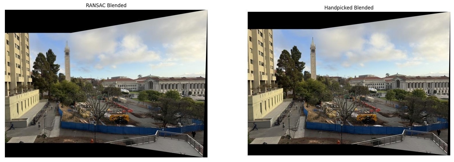
The automatic result doesn't align the images as well as the manual stitching again here, but this is probably the fault of my image taking skills. There are some slight artifacts in the image, such as the campanile on the left of the image being slightly off, and the walkway at the bottom of the image having blurry railings. However, the RANSAC stitching does so much better on the dead tree in the center of the image than the manual stitching. Maybe many of the good matches or homographies found by RANSAC did well on the tree in the center of the image, but the manual stitching did not. I think the automatic stitching struggles with the vast sky in this image, and maybe struggles with the repetitive texture of the buildings on the sides of the images.

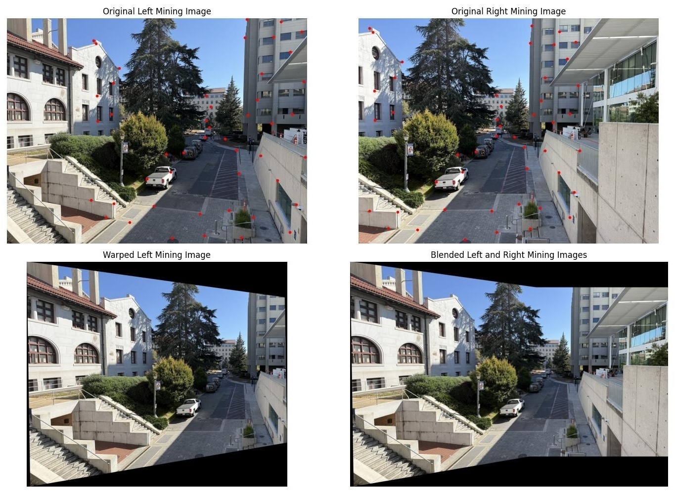
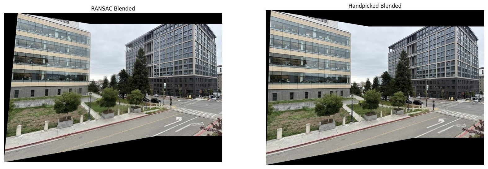
Mining Circle Comparison

Automatic stitching of the Mining Circle scene versus manual stitching.

The automatic result doesn't align the images as well as the manual stitching here. There are some slight artifacts in the image, such as the windows on evans hall being off. However, the automatic stitching does so much better on the food vans in the center of the image than the manual stitching. Generally, the automatic stitching does well on the center of these images. Again, there wasn't a ton of overlap in this image on the buildings, which is visually where most of the good corners are. The automatic stitching may also struggle here just because of my own ability to take images with good overlap and keep my hands steady to keep the center of projection fixed.

Good Automatic Stitching Results

After failure with the automatic stitching results on the part A images I used, I went out and took some more images that have less sky and more interesting and non repetitive texture. I used these images to test the automatic stitching pipeline. I use the same parameters as in the last section for the automatic stitching pipeline.

Automatic stitching of a street scene at the corner of College and Haste.

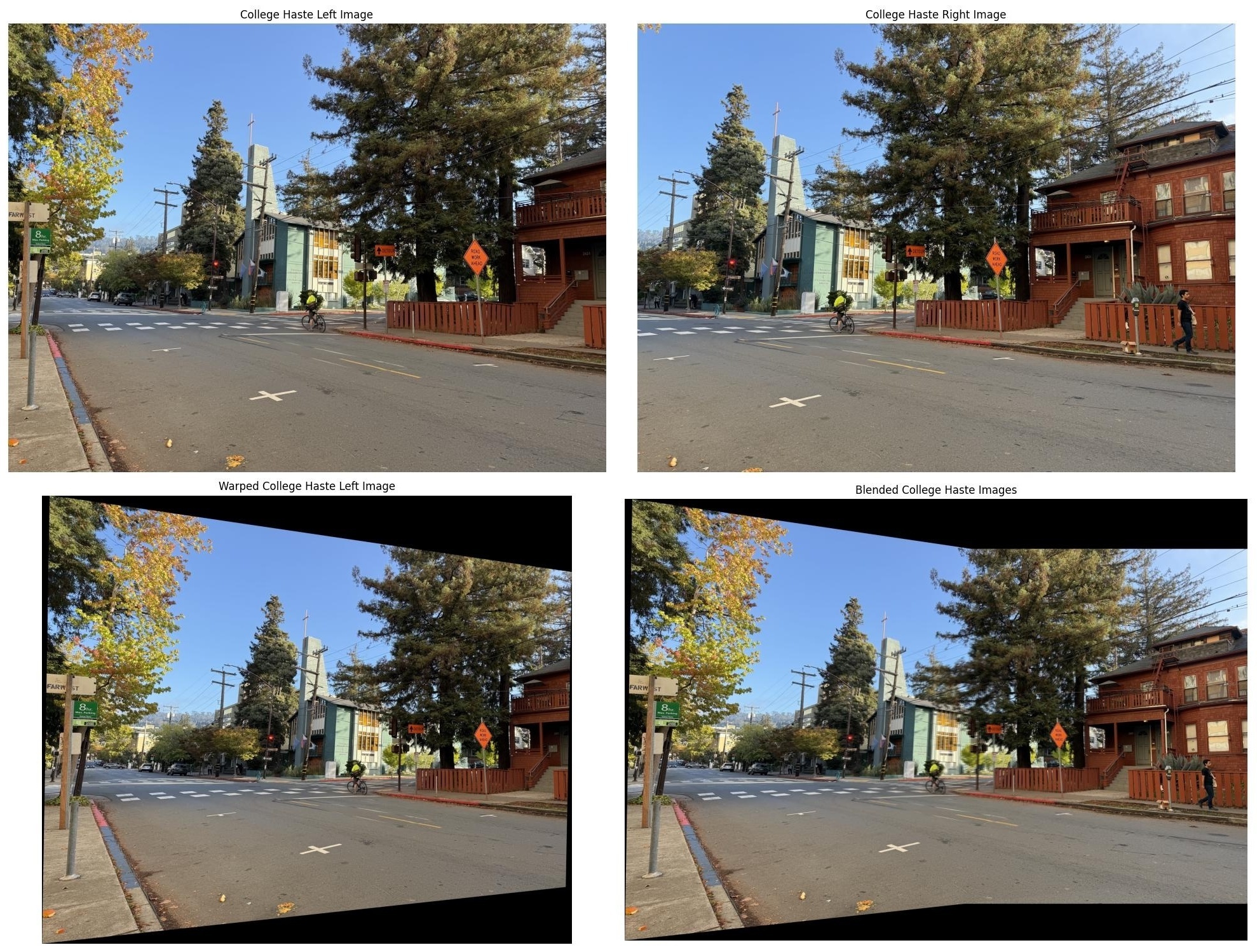
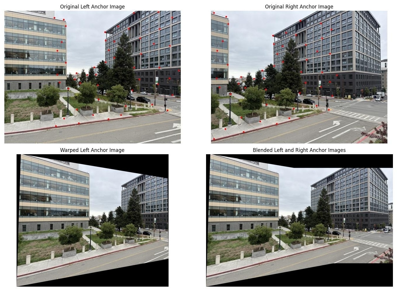
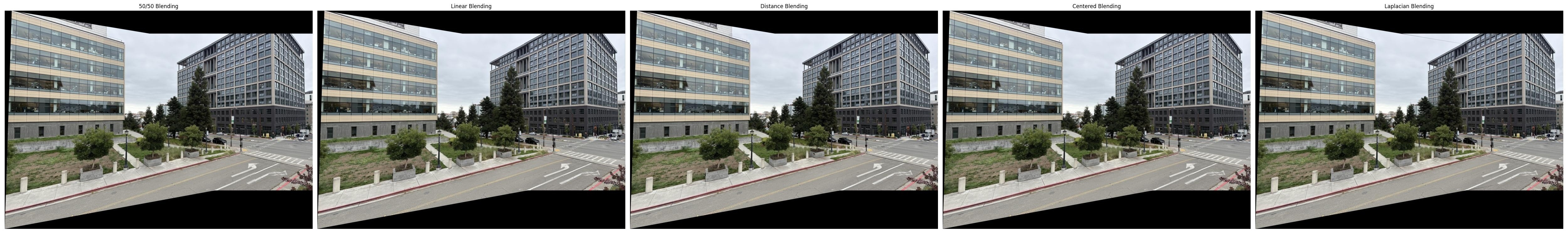
This image is a good example of the automatic stitching pipeline working well. There is a good amount of overlap between the images, and the automatic stitching is able to find good feature matches in the overlap. The result is a good blend of the two images, with little visible artifacts. The only visible artifact is the church building in the background of the image being slightly blurry, but once again this is probably the fault of my own image taking skills and keeping my hands steady to keep the center of projection fixed. The blending was done with centered radial falloff, but I also squared the alpha mask to get an even faster falloff. The blending method comparisons are shown below.

Blended mosaic of the college haste images using weighted averaging and various blending types.

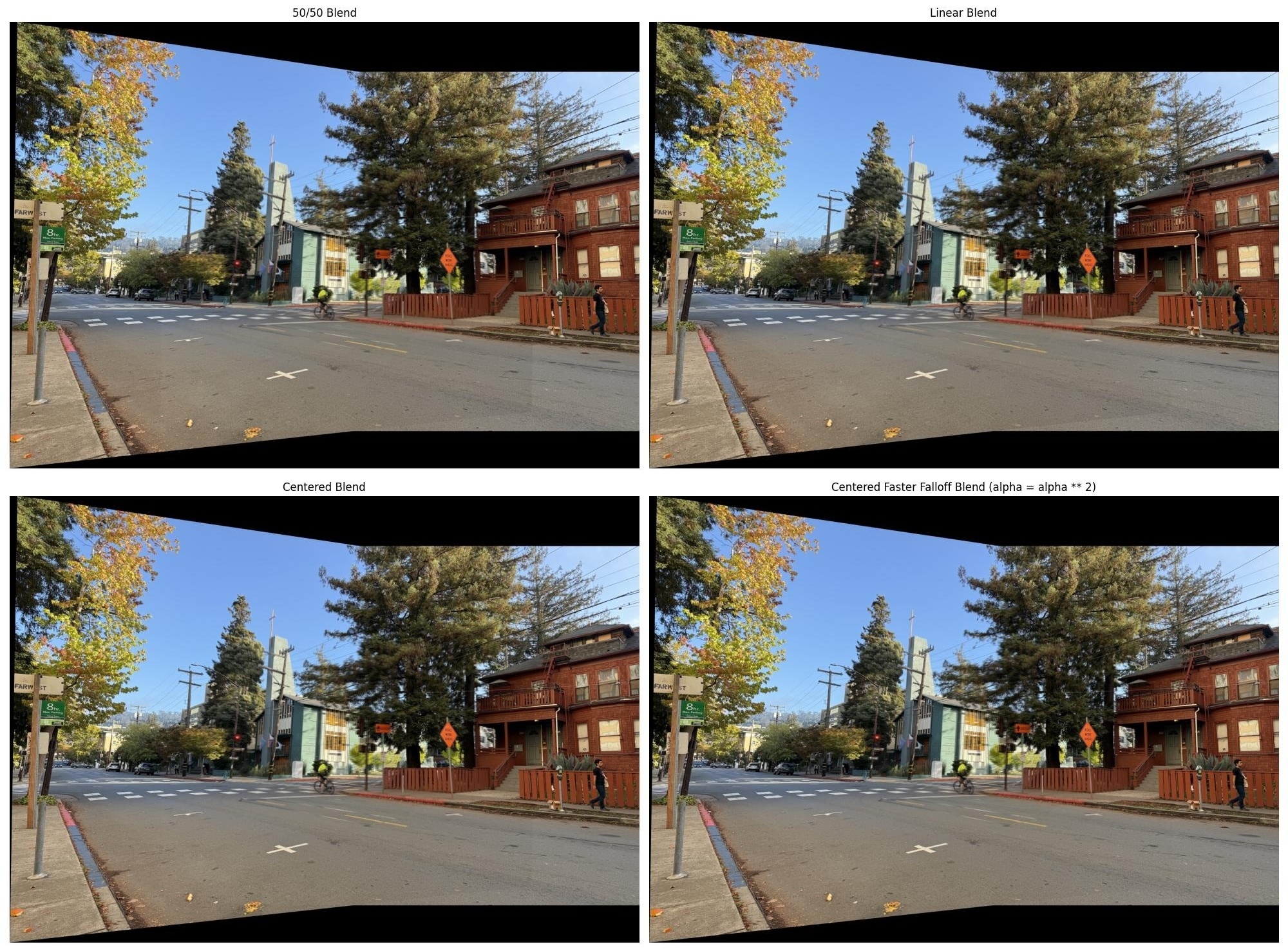
As you can see, the edges of the images are very visible without the centered radial falloff with a faster falloff. The linear falloff and the centered falloff look very similar with the same issue with the bottom right corner of the left image being prominent enough to see. This issue is solved by squaring the alpha mask, which gives an even faster falloff.

Automatic stitching of the images of the Unit 2 buildings. The two photos have different exposures, but we are able to blend out the edges.

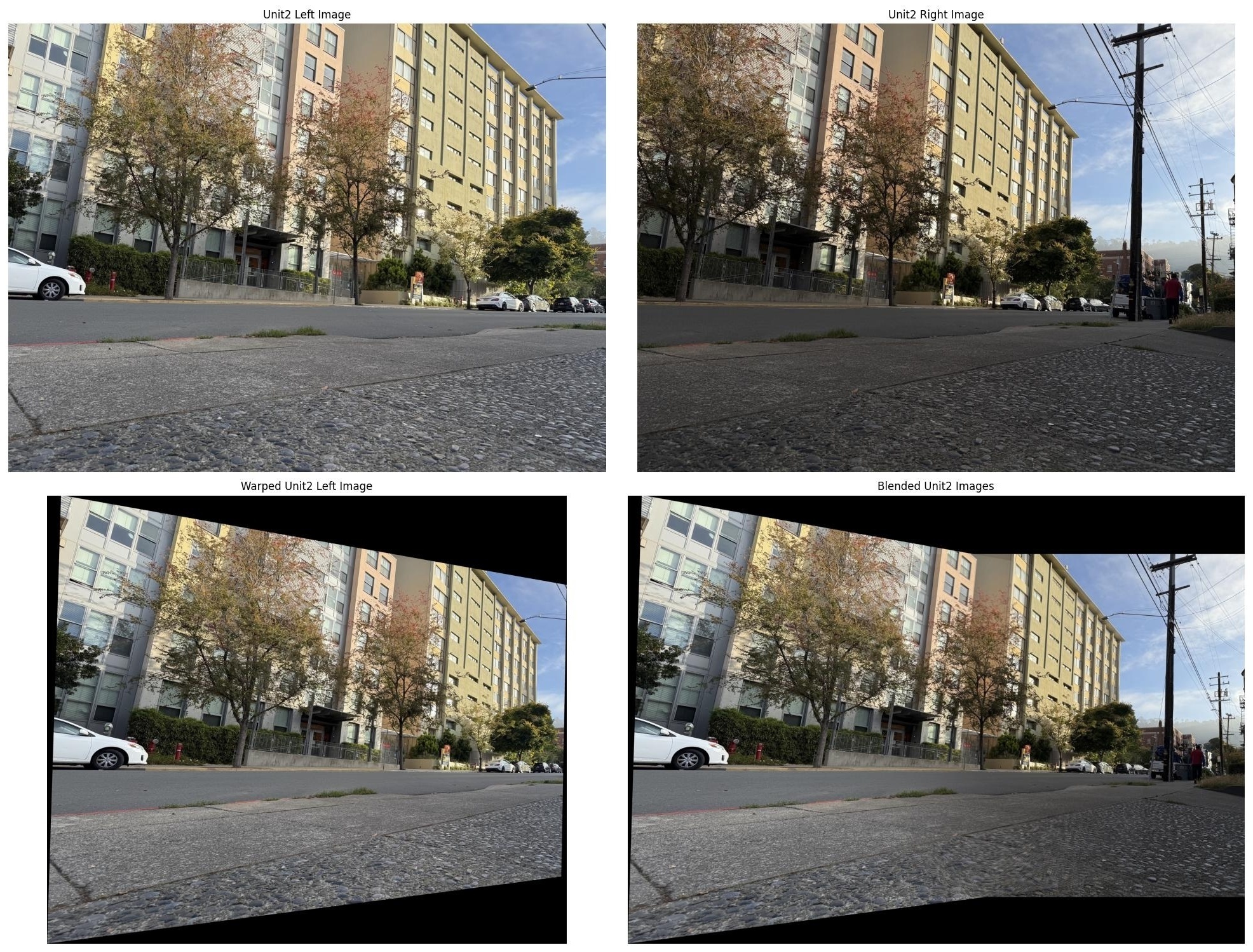
These images were taken pretty poorly, as the exposure is different between the two images. However, the automatic stitching is able to find good feature matches in the overlap, and the result is a good blend of the two images, with little visible artifacts. This image also has a good amount of repetitive textures, however, each building has different window sizes and many of the windows are varied with curtain textures, which seems to make the corners different enough to be able to match them well. The blending was done with centered radial falloff, but I also cubed the alpha mask to get an even faster falloff. The blending method comparisons are shown below.

Blended mosaic of the unit 2 images using weighted averaging and various blending types.

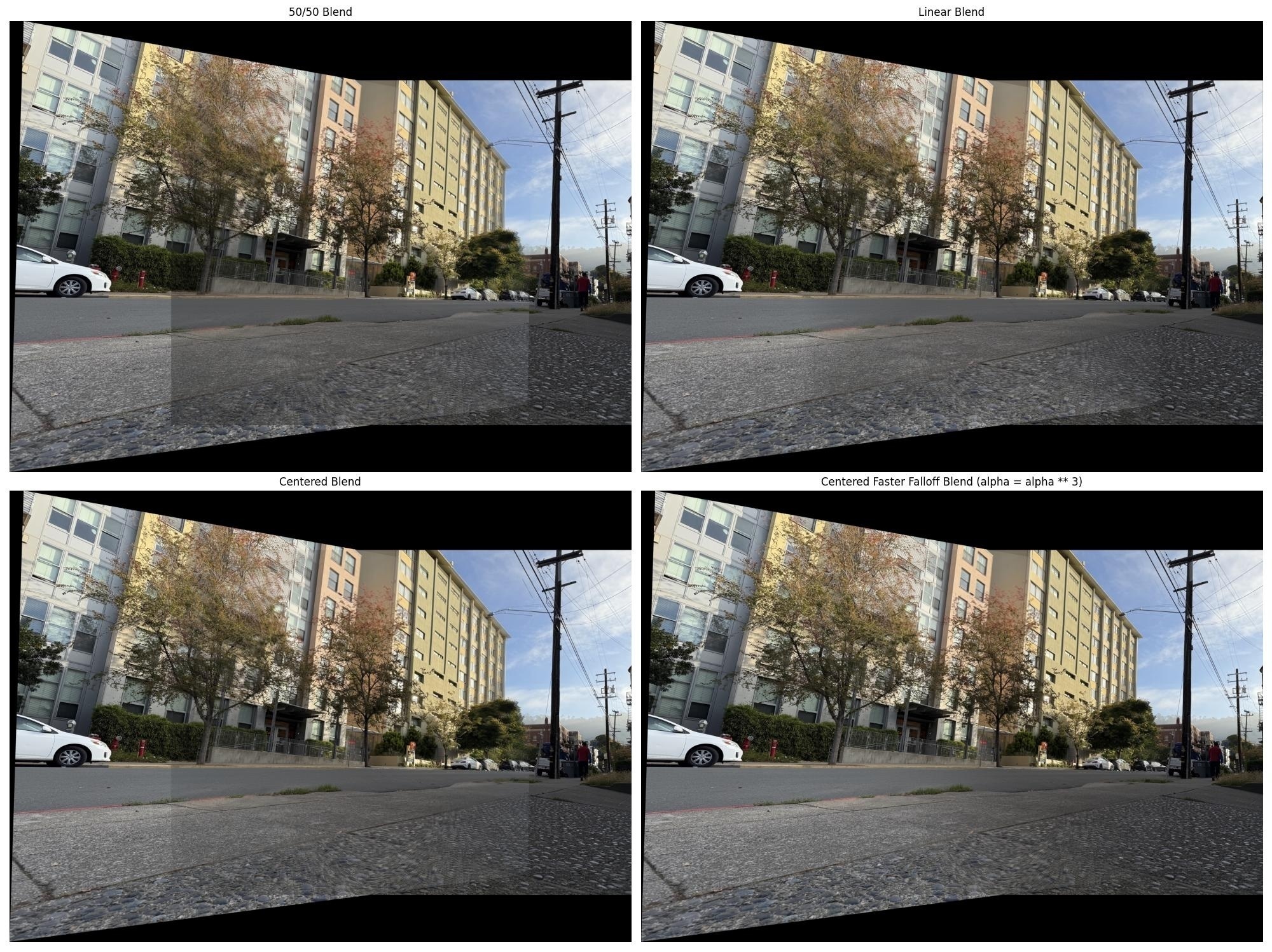
As you can see, the edges of the images are extremely visible without the centered radial falloff with a faster falloff of cubing. The linear falloff and the centered falloff look very similar with the same issue with all edges of both images being visible, because of the different exposures between the two images. This issue is solved by cubing the alpha mask, which gives an even faster falloff and helps to blend out the exposure differences between the two images.

Automatic stitching of the an apartment building courtyard. Originally, the bike on the right had some artifacting, but with some parameter tweaking, we were able to align it correctly.

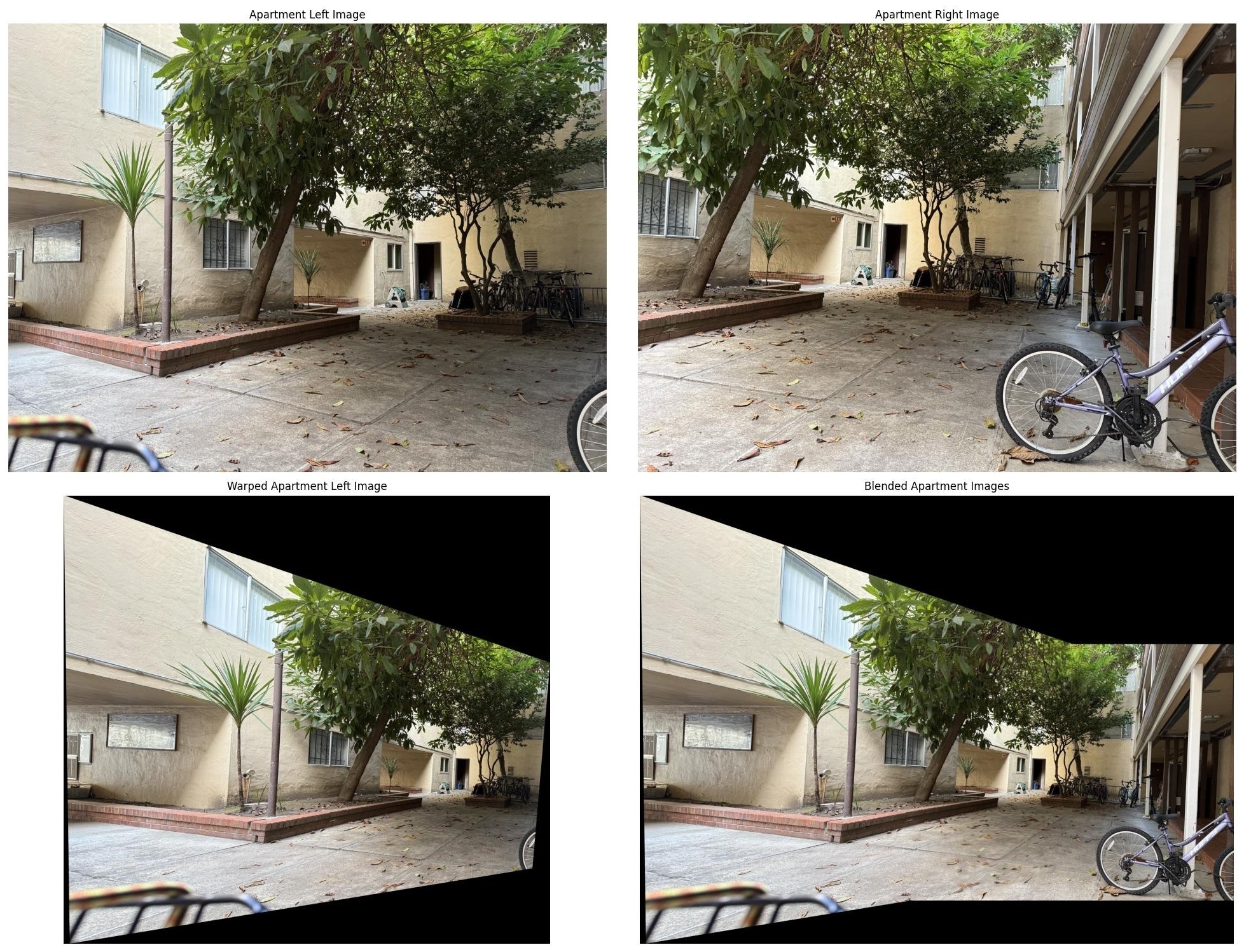
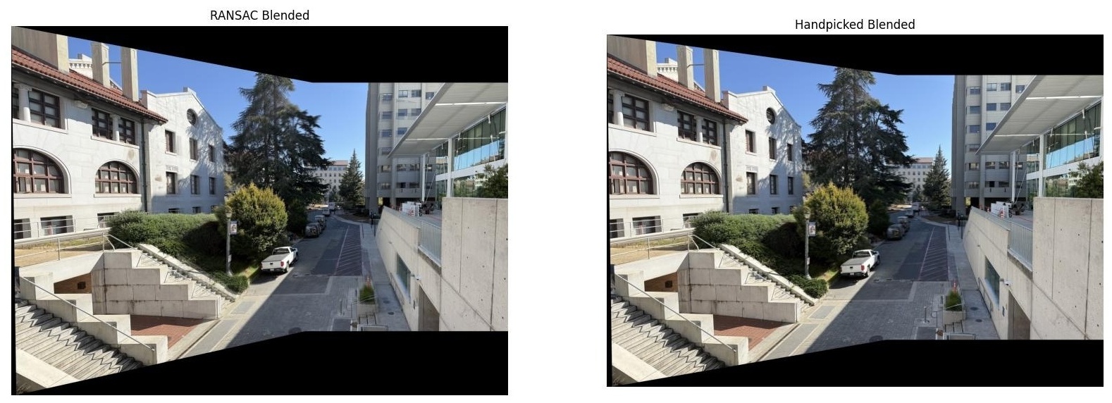
These images have little overlap, but the automatic stitching is able to find good feature matches in the overlap, and the result is a good blend of the two images. Maybe this is because it looks like some of the strongest corners could be in the overlap of the images, such as the dark doorway in the back, as well as some of the darkest windows being in the overlaping region. This image took some tuning to get the bike on the right to align correctly, but once again, this is probably the fault of my own image taking skills and keeping my hands steady to keep the center of projection fixed. But now the bike is aligned correctly and the only visible artifacting are some small leaves on the ground and some leaves on the tree in the background. The blending was done with centered radial falloff, but I also tried sqaring the alpha mask to get an even faster falloff. The blending method comparisons are shown below.

Blended mosaic of the apartment images using weighted averaging and various blending types.

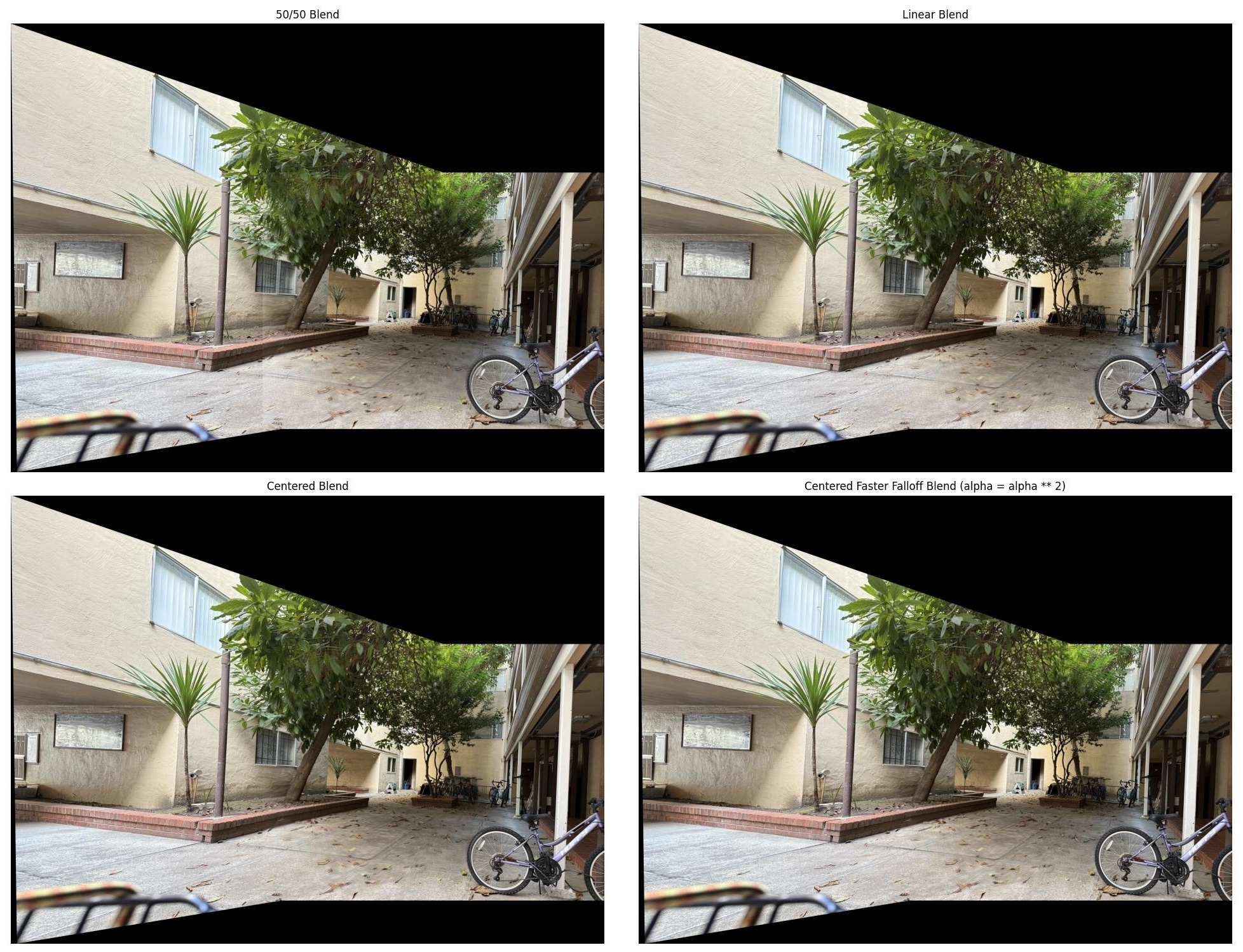
As you can see, the left edge of the image is pretty visible with 50/50 blending (no falloff), but the rest of the blending types look pretty similar and are able to blend out that edge. I tried squaring the alpha mask to get an even faster falloff, only to blend out a niticky edge in the far back of the image on the wall that is semi-visible in the other two blending methods. With the squaring method though, that edge is blended out well.