Project 2: Fun with Filters and Frequencies
The goal of this project is to gain a better understanding of filters and frequencies in images, and how we can use these to process images in unique and interesting ways.
Overview
In this project, we explore filters and frequencies in images. We first implement convolutions and create simple edge detectors with finite difference filters. We also explore image sharpening, hybrid images, and laplacian image pyramids. Using these tools we create fun hybrid images and multiresolution blended images!
Part 1.1: Convolutions from Scratch
In this part, we implement convolutions from scratch using nested for loops. We first create a simple function that uses four nested for loops to perform a convolution. In this implementation, we naively sum each individual product for each pixel of the image with the kernel. We then create a function that uses two nested for loops with numpy operations to perform a convolution. In this implementation, we instead use np.dot to perform the convolution for each window slide of the kernel on the image. For both of these implementations, we pad the image with zeros based on the size of the kernel. We also flip the kernel to make sure we are performing "real" convolution. We then compare the results of these two functions and scipy.signal.convolve2D for a simple grayscale image of me and a box filter.
All of these methods used 0 padding for the image, thus treating the edges of the image the same. We use scipy.signal.convolve2D with mode='same', boundary='fill', and fillvalue=0 to perform the convolution the same way. I double checked that all of these methods gave the same results by running np.allclose on the results of the three functions. Code snippets are shown below.
def conv_with_four_loops(image, kernel):
    kernel_h, kernel_w = kernel.shape
    padding_h, padding_w = kernel_h // 2, kernel_w // 2
    image_padded = np.pad(image, ((padding_h, padding_h), (padding_w, padding_w)), mode='constant')
    kernel_flipped = np.flip(kernel, axis=(0, 1))
    result_image = np.zeros_like(image)

    for i in range(image.shape[0]):
        for j in range(image.shape[1]):
            for k in range(kernel_h):
                for l in range(kernel_w):
                    result_image[i, j] += image_padded[i + k, j + l] * kernel_flipped[k, l]

return result_imagedef conv_with_two_loops(image, kernel):
kernel_h, kernel_w = kernel.shape
padding_h, padding_w = kernel_h // 2, kernel_w // 2
image_padded = np.pad(image, ((padding_h, padding_h), (padding_w, padding_w)), mode='constant')
kernel_flipped = np.flip(kernel, axis=(0, 1))
result_image = np.zeros_like(image)
for i in range(image.shape[0]):
for j in range(image.shape[1]):
result_image[i, j] = np.dot(
image_padded[i:i+kernel_h, j:j+kernel_w].ravel(),
kernel_flipped.ravel()
)
return result_image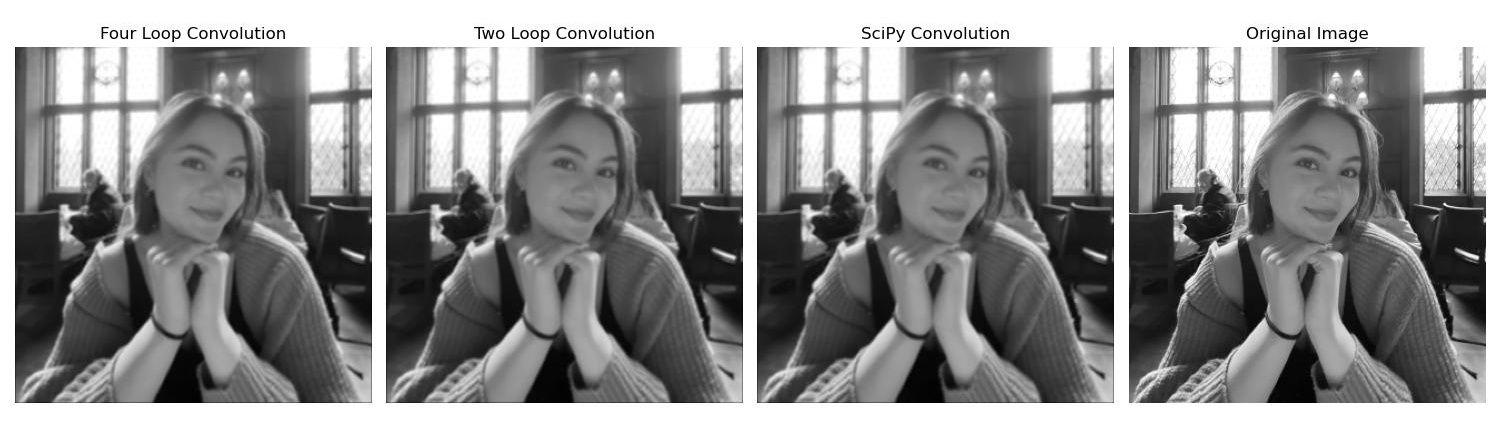
The results of the convolutions are shown above. As we can see, the results of the three functions are the same. However, these functions are not the same speed. The four nested for loop function is the slowest, followed by the two nested for loop function, and then the scipy.signal.convolve2D function. Four loop time: 0.399 seconds, Two loop time: 0.169 seconds, SciPy time: 0.003 seconds. The exact times varied slightly between runs, but the relative times were the same (i.e. four loop was always slower than two loop, and two loop was always slower than scipy).
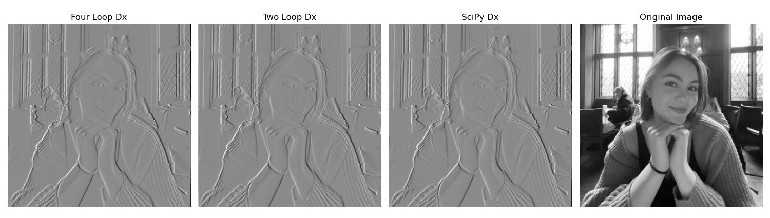
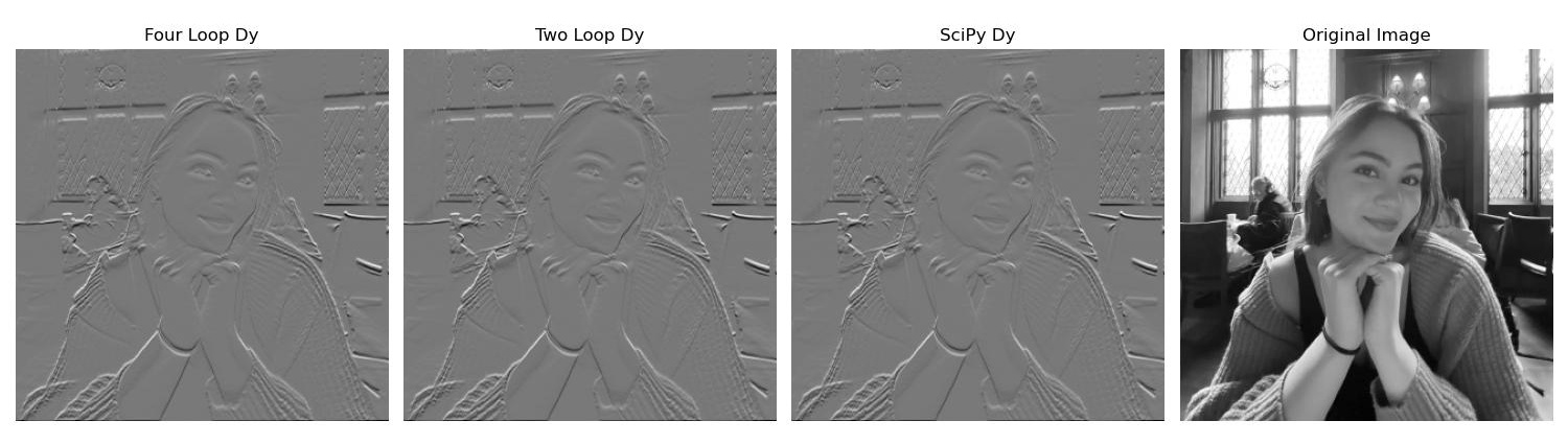
We also convolve the image of me with the finite difference filters Dx and Dy. Dx = [1, 0, -1] and Dy = [1, 0, -1]^T, which give us the partial derivatives of the image in the x and y directions respectively. Again, the results of the three functions are the same. These images are shown below.
Part 1.2: Finite Difference Operator
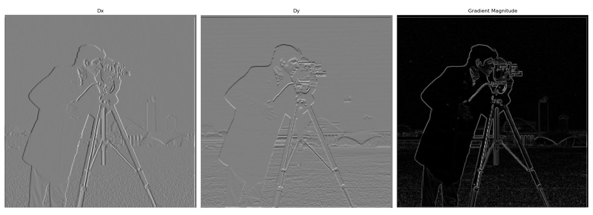
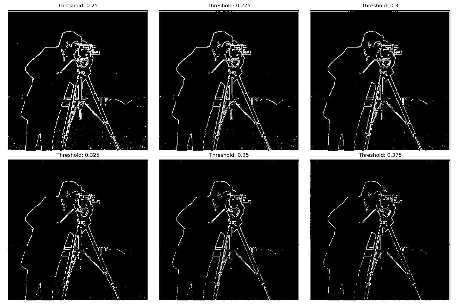
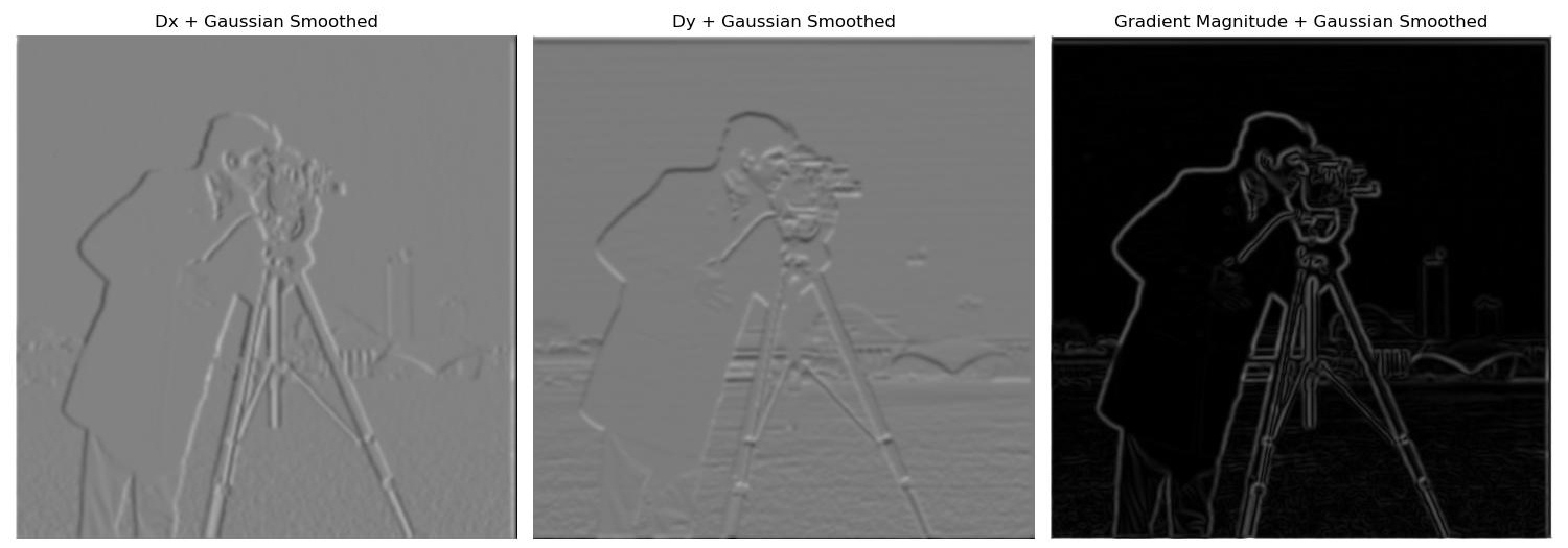
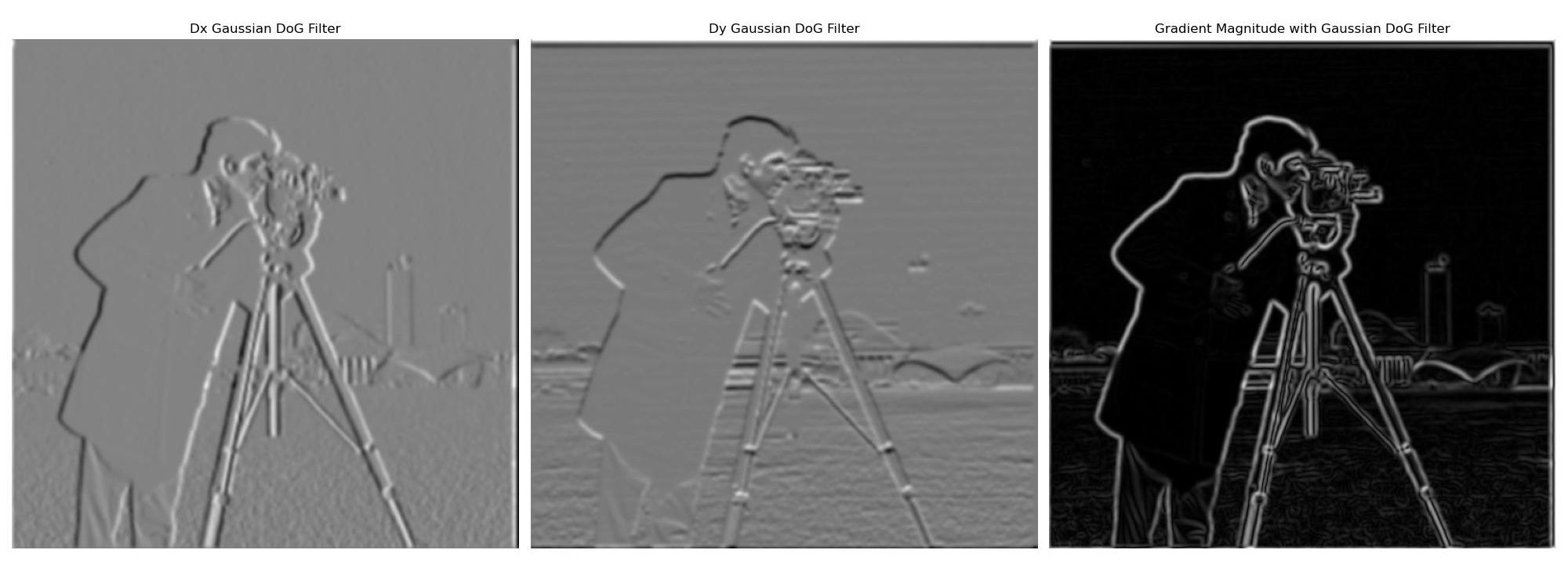
First, we show the partial derivatives in x and y directions of the cameraman image (using finite difference filters Dx, Dy again). Using these partial derivatives, we can compute the gradient magnitude image with sqrt((partial derivative image in x direction)^2 + (partial derivative image in y direction)^2). We then use the gradient magnitude to create a simple edge detector by binarizing the gradient magnitude image with a constant threshold. We take the binarized image with (gradient magnitude image > threshold). With this method, it is difficult to trade off between noise and edge detection. There is a lot of grain in these images.
The threshold I chose as the best trade off was 0.325. With this threshold, most of the noise at the bottom of the image is removed, but we can still see most of the back leg of the tripod and the smaller buildings at the back. There is still some noise in this image. I show the results of all of the best different thresholds I tested below, including 0.325.
Part 1.3: Derivative of Gaussian (DoG) Filter
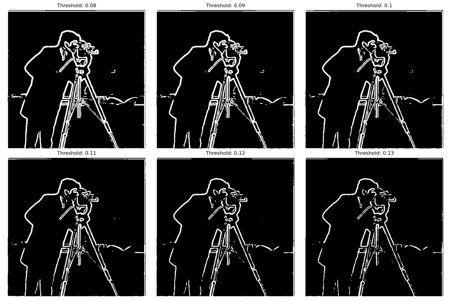
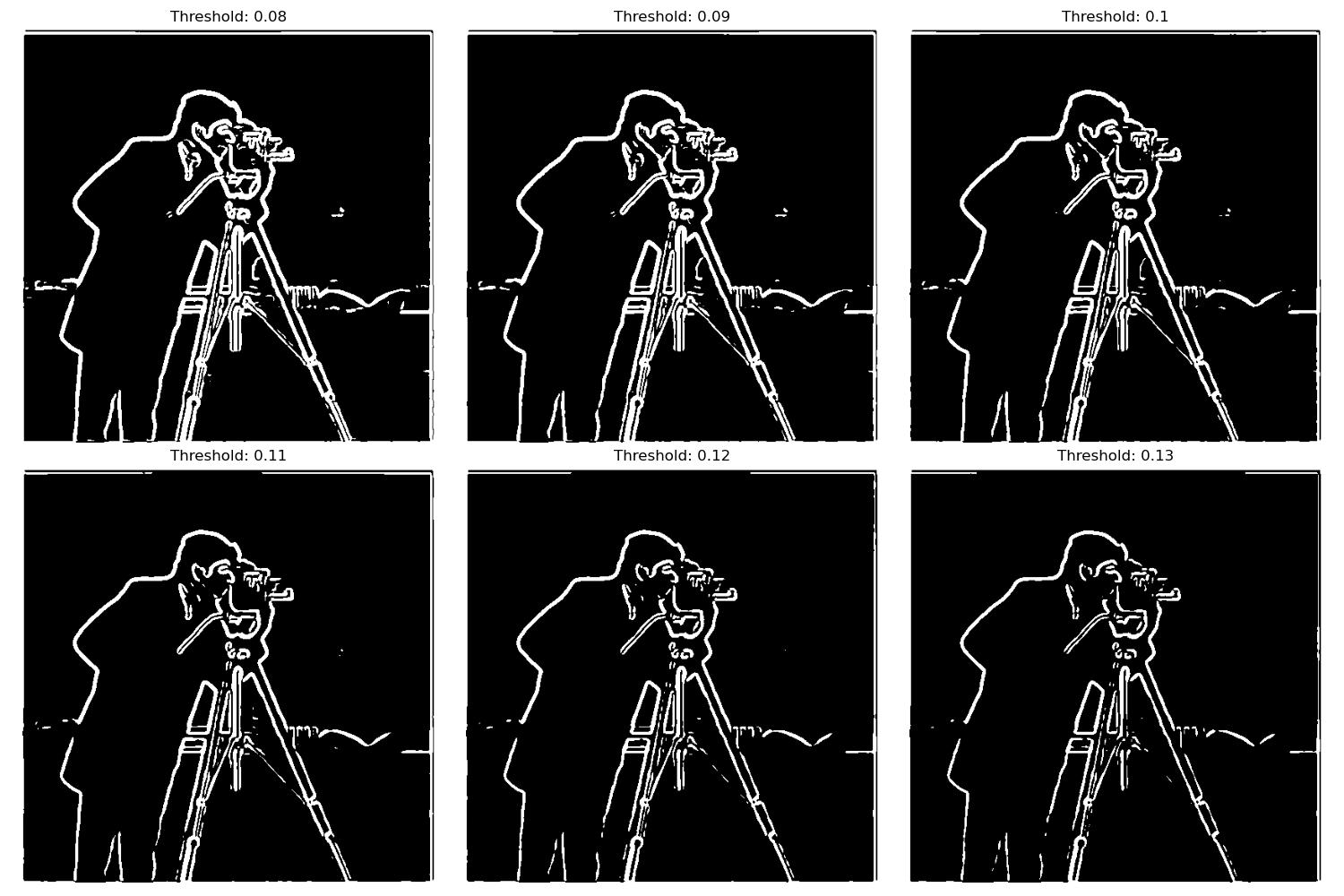
Next, we try to improve this edge detector by first convolving the image with a Gaussian filter to blur the image, and then computing the gradient magnitude of the blurred image with the same method as above. We then use the gradient magnitude of the blurred image to create a simple edge detector by binarizing the gradient magnitude image with a constant threshold again. We use a Gaussian filter with a sigma of 2 and a kernel size of 13, for some, but not too much blurring. I choose a threshold of 0.08 to be the best under this method, as we don't lose the mouth of the cameraman or the top of the building in the back. There are still one or two grains left, but it is a much cleaner image. Overall, the results for this method are much cleaner than just the finite difference method. Most of the noise is removed already in the gradient magnitude image, because of the blurring. We compare different results of the new edge detector with different thresholds below, including 0.08.
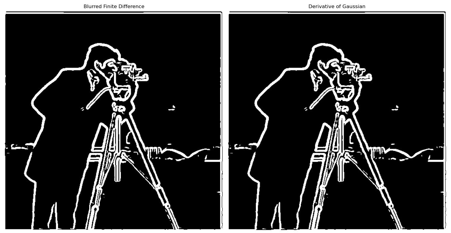
Now we combine the Gaussian and finite difference filters together to get one kernel to convolve with the image. The new DoG kernels are created by convolving the Gaussian and finite difference filters together. We use a kernel size of 13 and a sigma of 2 again to keep results consistent. The results of the partial derivatives as well as the edge detector are shown below. We can see that the edge detector gets the same results as when we convolved the image with the Gaussian and finite difference filters one at a time. The best threshold is still 0.08.
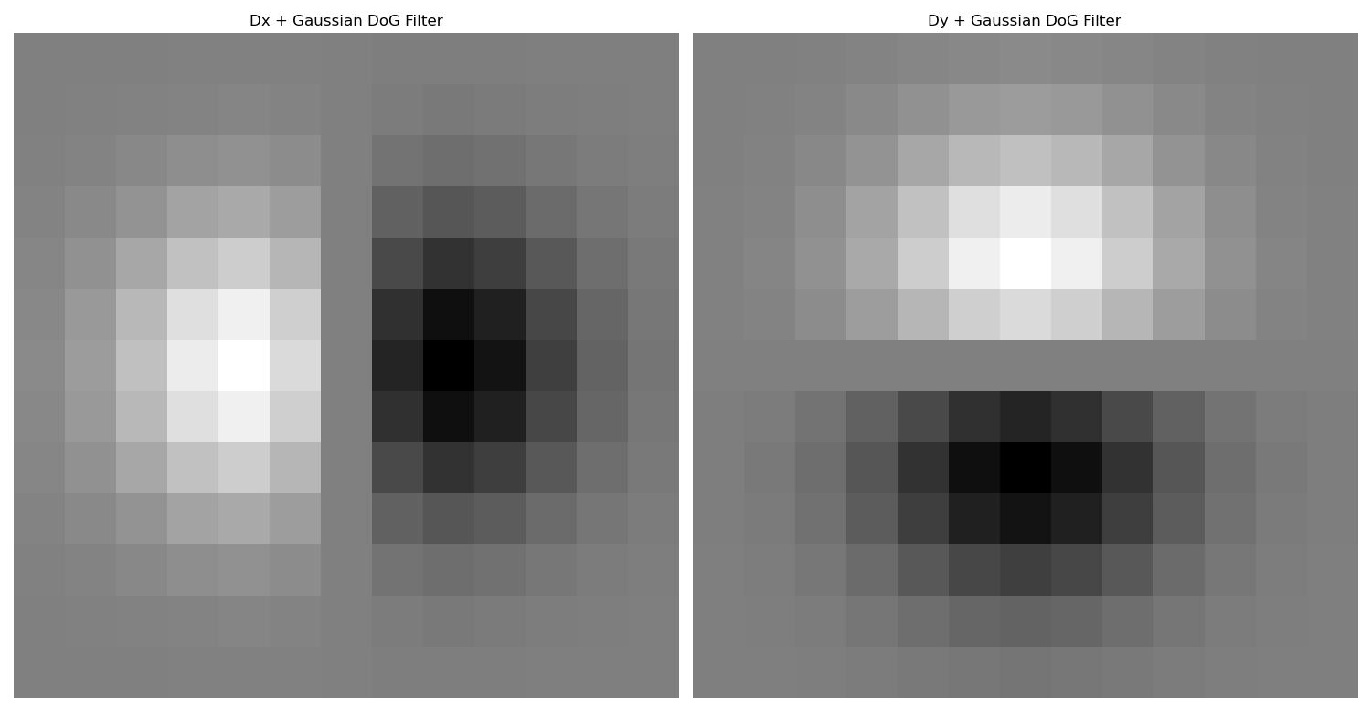
The results of the edge detector with the DoG filter and the original blurred method come out to be the same. I display a comparison image below of the detected edges with both methods (both with the same threshold of 0.8).
Part 2.1: Image Sharpening
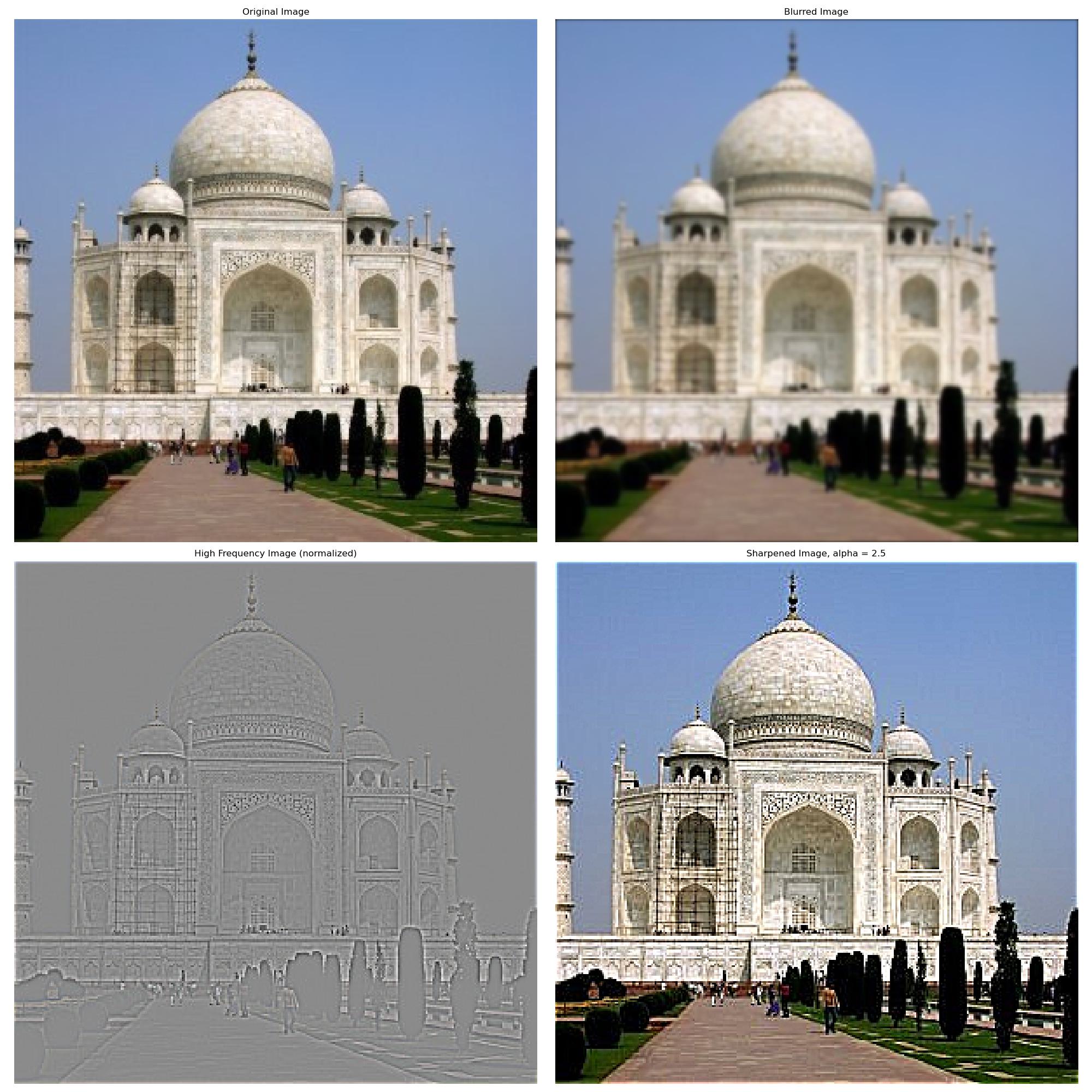
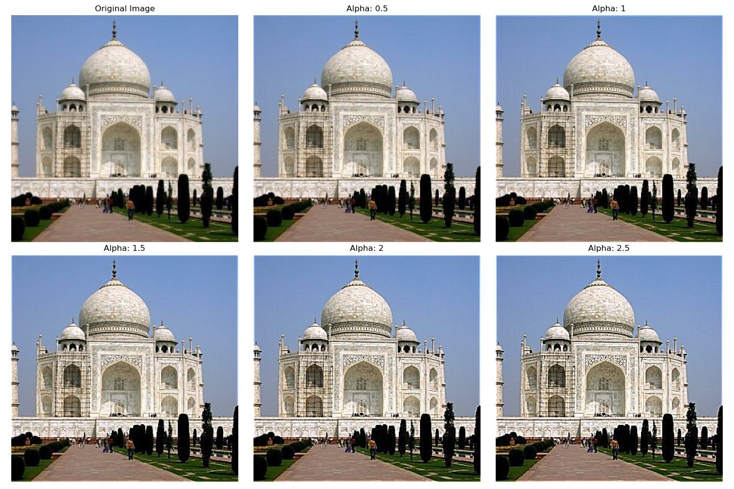
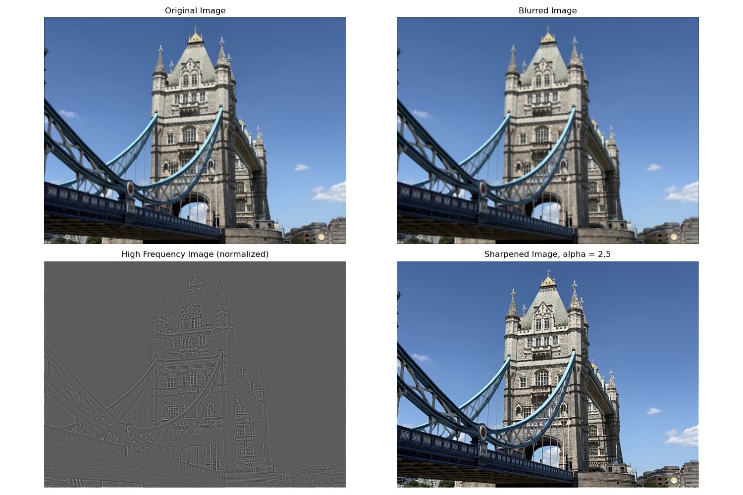
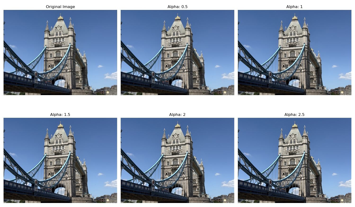
In this part, we explore image sharpening. We first create a function that sharpens an image by convolving it with a unsharp mask filter. This filter is essentially adding the high frequency back to the original image. We can do this by blurring the image with a gaussian kernel and then subtracting the blurred image from the original image to get the high frequency image. We then add the high frequency image back to the original image with some constant value alpha to get the sharpened image. In practice, we can calculate just one filter, the unsharp mask filter, by subtracting alpha times the gaussian kernel from (1 + alpha) times the unit impulse. Our gaussian kernel is 7x7 with a sigma of 1 for minimal blurring which means we are only adding back the highest of frequencies. We then convolve the image with this filter with various values of alpha to get the sharpened images. We then compare the results of these images with the original image.
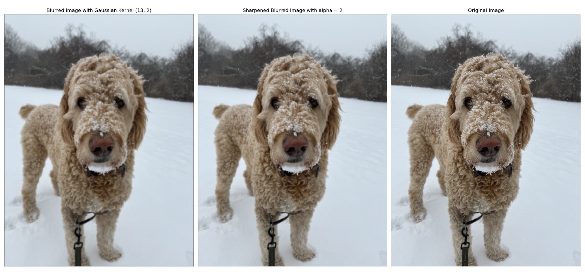
Now, we try the same thing on a blurry image. I blurred an image of my dog with a gaussian kernel 13x13 with a sigma of 2, then sharpened that image. My dog image was quite big, so I needed to blur it more to visibly see the sharpening process on the blurry image. The results are shown below. As you can see, the image does look more sharp, but there are some details in the original image that were lost when we blurred it that couldn't be recovered by the sharpening process. This is because the blurring removes the highest frequency components of the image, and the sharpening process can only add back the high frequencies that are still present in the image.
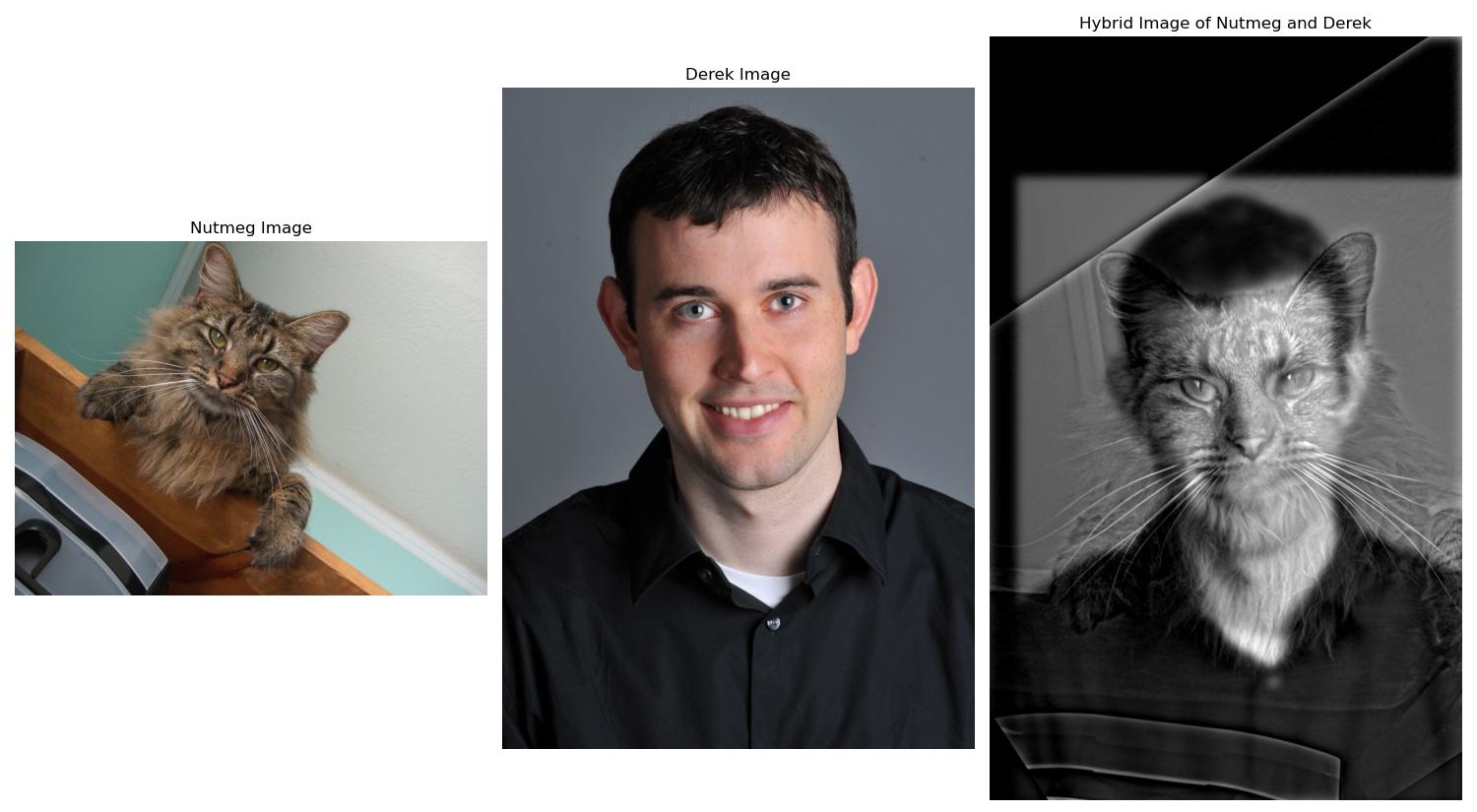
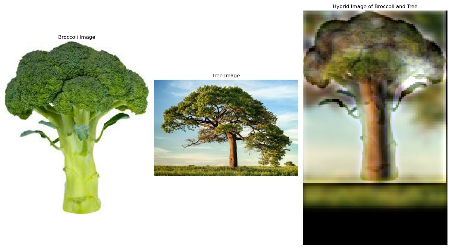
Part 2.2: Hybrid Images
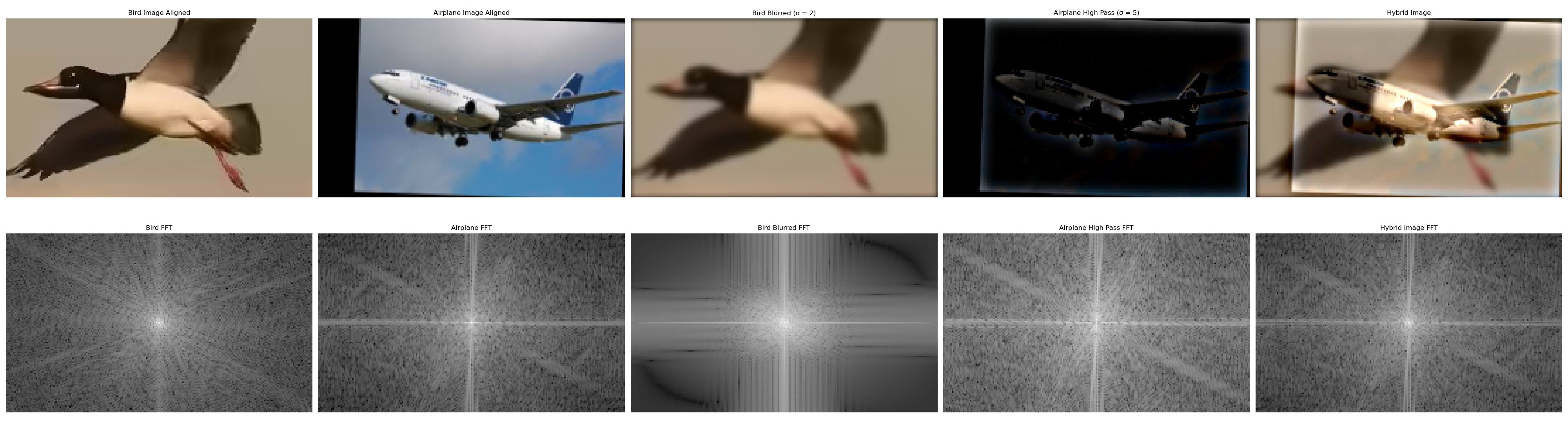
In this part, we create hybrid images. We first have to align the two images by selecting two points in each image for alignment. The images are then rotated and resized to match these two alignment points we selected for each image. Then, we convolve the two images with their respective gaussian kernels to get two lower frequency images. We subtract one image from its original to get a high frequency image. We then add the low and high frequency images together to get the final hybrid image. For each example, the original images and the hybrid image are shown. For the example with the bird and the airplane, the fourier transform of the original images, blurred and high frequency images, as well as the hybrid image are also shown. The gaussian kernels are chosen with some trial and error, trying to strike a good balance to make the hybrid images look good. Thus, some of the sigma values are not the same for each image and were chosen empirically.
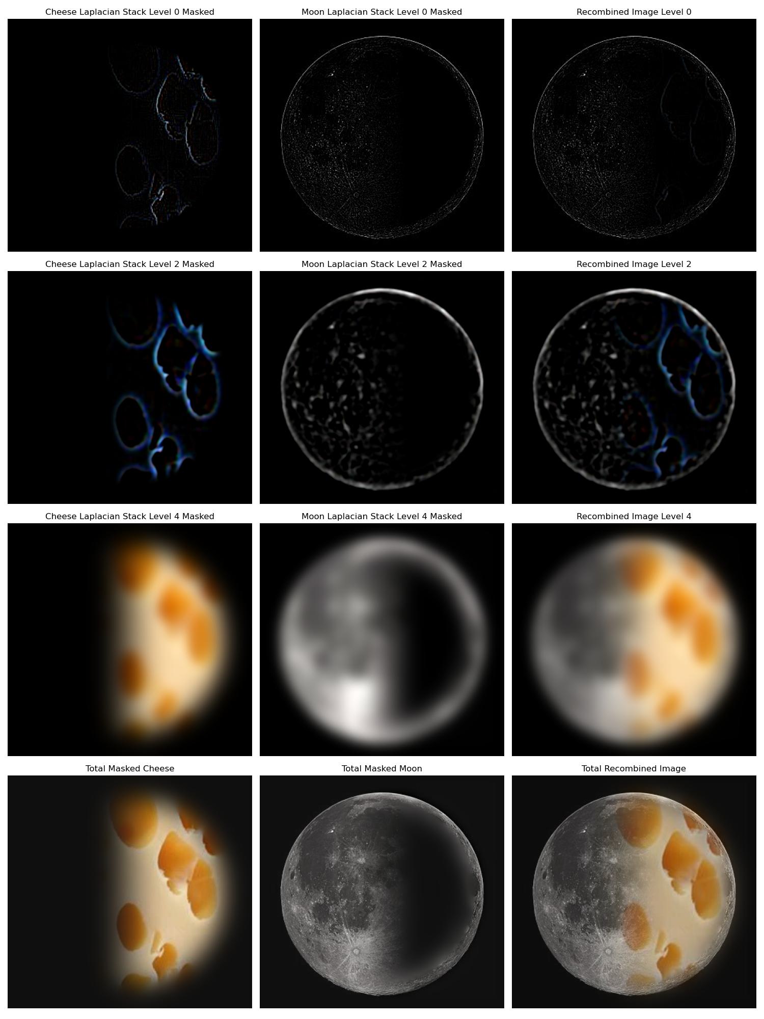
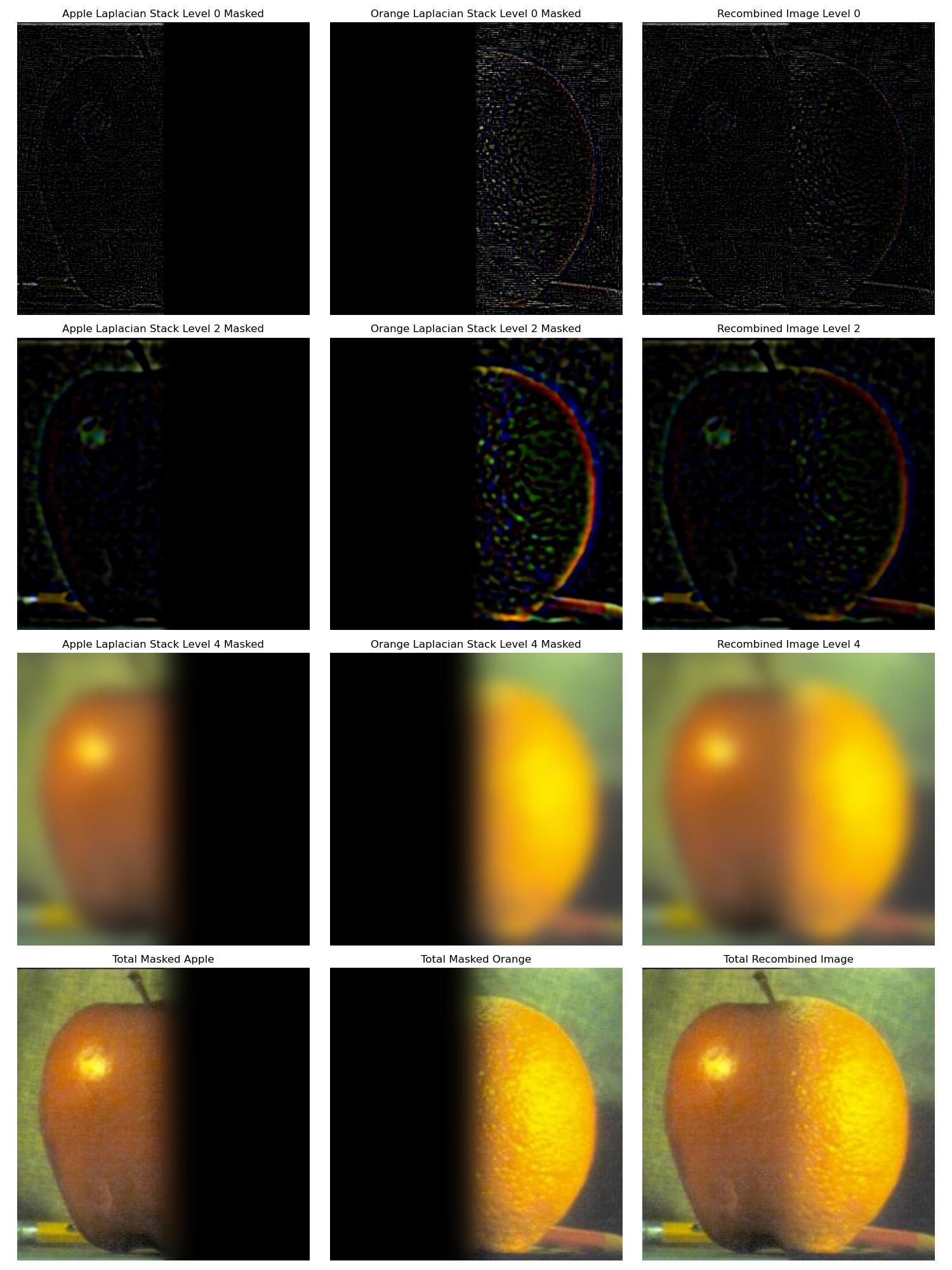
Part 2.3: Gaussian and Laplacian Stacks
In this part, we create Gaussian and Laplacian image stacks. We first create a function to create a gaussian stack of an image. This is achieved by convolving the image with a gaussian kernel and then increasing the sigma and the size of the kernel by some factor to get the next layer. This results in a list of images, each with the same size, but each more blurry than the next. We then create a function to create a Laplacian stack of an image. This function calls the former function to create a gaussian stack, then subtracts the neighbors in the gaussian stack from each other to get individual frequency bands, which is the the Laplacian stack. The bottom layer of the Laplacian stack is the same as the lowest frequency layer of the gaussian stack.
We create a laplacian stack for each reference image. We also create a gaussian stack for the mask image that we will use to blend the two images. We use a gaussian sigma starting at 1 doubling with each layer for each stack. We recalculate the gaussian kernel size at each layer to be 6*sigma + 1. We recreate the image from Figure 3.42 in Szeliski's book draft, Computer Vision: Algorithms and Applications. This is done by multiplying layers 0, 2, 4 of the laplacian stack with the respective layers of the mask gaussian stack and then adding them together. The apple layers get multplied by the mask layers while the orange layers get multiplied by 1 minus the mask layers. We then display the resulting images.
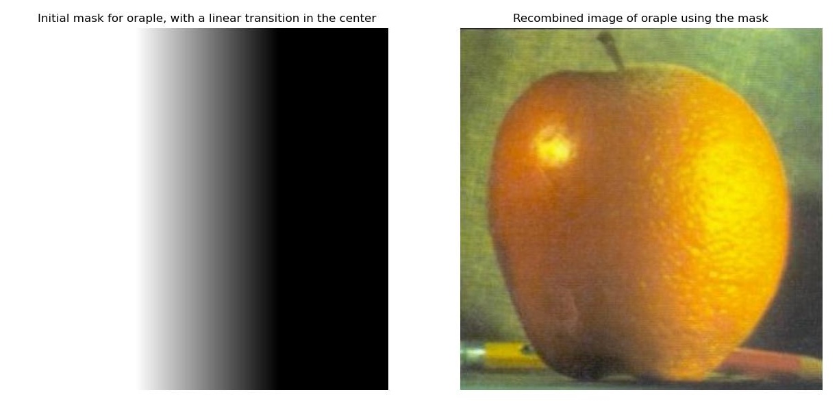
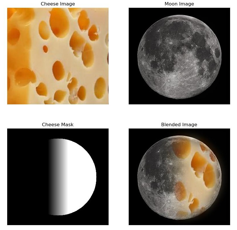
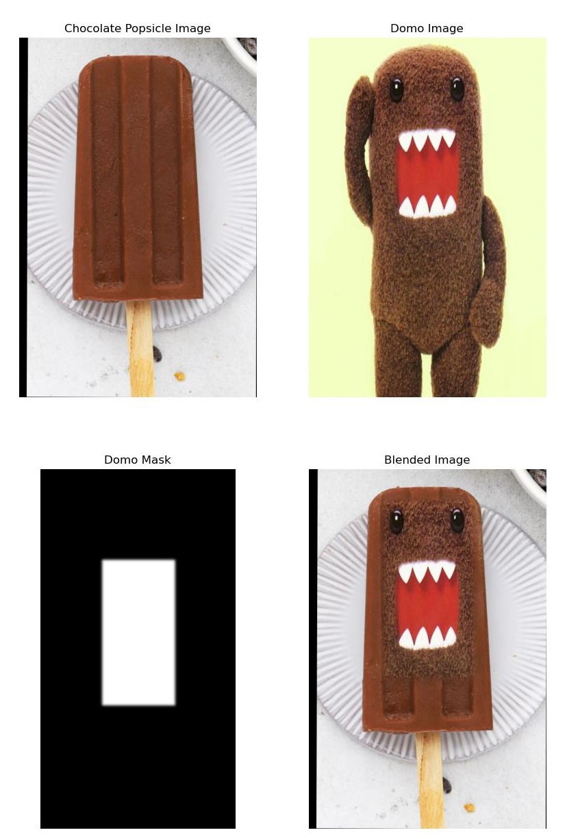
Part 2.4: Multiresolution Blending
In this part, we blend two images together using the same multiresolution approach as described in the previous part. In this part, I made the mask images of interesting shapes, or in the case of the orange and apple, I made the transition in the center of the image linear to make the blended result look smoother. The results and masks are shown below.